L'autopilot analyse l'heure, ton jour de plan, ton streak et tes weaknesses.
📝
Test mémoire — hier (J0)
Évalue ta rétention sur les concepts vus hier (3-5 questions rapides)
⏮
Tu as fait une séance hier ?
Si oui, restaure la validation (perdue après cache cleared par exemple). Ça remettra ton plan en cohérence (today = J2).
0
🔥 Streak
0
Cartes 7j
0
Minutes 7j
0/7
Cohérence 7j
📅 Tes 90 derniers jours— actifs sur 90
LMVD
MoinsPlus
Best use of the next 20 minutes
Loading your next action...
Checking due cards, weak themes and exam practice history.
🧭Exam mode — concrete route▼
Level 1 · 20 minutesRead the exam sheets for sessions 2, 3, 5, 6. Objective: know how to recognize the model and formulas without calculating.
Level 2 · 45 minutesManipulate the interactive graphics, redo the movements by hand, then explain the intuition in one sentence.
Level 3 · 90 minutesDo the standard exercises, then the SRS flashcards. Objective: transform concepts into exam reflexes.
⚡
Quick Revision
All key ideas in 5 minutes
🃏
Flashcards
Spaced repetition study
✅
Quiz
Test your knowledge
📊
Interactive Graphs
IS curve, multiplier, investment
🗺️
Models Map
How every model connects
🧪
Exam Simulator
Timed prompts and corrections
🧩
Coverage Map
Chapters, sources, exercises, gaps
⏱️
Revision 30/60/90
Plan filtered according to your weaknesses
🎯
Exam mode only
Formulas, graphs, topics, pitfalls
📝
Mock Exam
Balanced 75-minute paper
📈
Graph Drills
Curve shifts with correction
🧮
Numeric Drills
Calculations with auto-correction
⚠️
Top 10 Exam Traps
Mistakes to avoid under pressure
🎯
Weakness Dashboard
Prioritize what to revise next
🕯️
Exam Eve
Last-hour formulas and traps
💾Backup or restore my progress▼
Your progress (SRS flashcards, quiz scores, numeric drills, mock exams) lives in browser localStorage. If you switch device or clear your cache, it's gone. Download regularly and import on the other device.
Backup status loading...
📅 Planning de Révision (3 semaines)
Programme jour par jour jusqu'à l'examen. Coche chaque jour à mesure que tu avances.
J-—
🔄Les jours validés dans Due Today apparaissent automatiquement en verts ici. Tu peux aussi cocher manuellement.
📍 Le plan démarre aujourd'hui. La date d'examen est ajustable — par défaut J21.
🎯 Path to 20/20 — Audit & Plan en 3 semaines
De zéro à 20/20 — chemin précis basé sur un audit complet du projet et des Teaching Notes.
🎯 3 messages essentiels
1
The content is 85% ready. Three weeks are enough if you follow the 21-day plan without skipping the mock exams.
2
2 structural risks fixed in this update: (a) the UIP formula typo, (b) the main translation artefacts.
3
The behavioral layer makes the difference. Keyboard shortcuts + streak + P1-P8 habits move you from 14 to 17. Missing Naef sessions + deeper Open Economy practice move you from 17 to 20.
T7Mode impression (@media print) + bouton 🖨️ flottant★★★★Small✓ Fait
T8Fix mobile : classe .alain-session-section responsive★★★★Small✓ Fait
T9Auto-export hebdo localStorage (anti-perte Safari)★★★Small✓ Fait
T105 drills numériques supplémentaires (Okun, BB, IS, mkt i, PPP)★★★Medium✓ Fait (now 10 drills)
T11UIP interactif + Mundell-Fleming 3-panels (sec-openeco)★★Large✓ Fait
T12Lazy-load galleries (55 images lazy)★★Small✓ Fait
T13Prompt "Pourquoi ?" après rating Good (overlay)★★★Small✓ Fait
T14Split en modules (macro-modules/)★LargeMaintenance
💡Habitudes pratiques (P1-P8) — ce qui sépare 14/20 de 20/20▼
P1Handwrite each IS-LM-PC + Phillips graph BEFORE opening the solution. Graders score the drawing, not the click.★★★★★SmallCritical
P2Enable Blind mode for every flashcard session.★★★★SmallHigh
P3Use a fixed daily 90-minute block + macOS notification.★★★★SmallHigh
P4Say one why sentence out loud after each exercise.★★★★SmallHigh
P5Record every mock-exam score in a paper notebook next to the laptop.★★★SmallMedium
P6No new content after J19 — consolidation and sleep only.★★★★★SmallCritical
P7Teach one concept to someone at J14 and J20 — Feynman technique.★★★★SmallHigh
P8Imprimer la formula bank (une fois T7 implémenté) et la garder sur le bureau 3 semaines★★★SmallAprès T7
📍 Pour démarrer maintenant
Ouvre → calendar et règle ta date d'examen exacte
Aujourd'hui = J1. Ouvre → alain-s1 pour 90 min
Active le Blind mode en haut du deck flashcards principal
Garde cette page (Path to 20/20) ouverte dans un onglet — c'est ta carte
⏰ Ta journée de révision
AUJOURD'HUI
—
—
✅
Séance validée
—
0%
Tâches du jour0 / 0 cochées
Streak 🔥0 jours
🎯
Mission du jour
⏱ —
ℹ️Où est le Main deck (150 cartes) ?
Le Main deck a son propre onglet : 🃏 Flashcards (SRS) dans la sidebar.
Les decks ci-dessous sont les decks thématiques par session (Naef S1-S6 + Économistes).
🃏Cartes dues — decks thématiques (sessions + économistes)0
📝Note du jour (optionnel)
Coche toutes les tâches puis valide pour enregistrer ta progression et garder ton streak 🔥
💡 Comment utiliser cette vue
Coche chaque tâche au fur et à mesure → l'anneau se remplit
Navigue avec ⬅ / ➡ pour voir hier (passé) ou demain (planifié)
Priorité aux decks rouges (>20 cartes dues)
Valide la séance en fin de journée pour maintenir le streak 🔥
J—
⭐ Cartes étoilées
Tes cartes marquées comme difficiles. Révise-les en priorité avant l'examen.
💡Comment ça marche
Clique sur l'icône ⭐ en haut à droite d'une flashcard pour la marquer.
Ces cartes apparaissent ici, groupées par deck. Idéal pour la révision finale J19-J20 sur les pièges qui te résistent.
⚙️ Settings
Personnalise l'interface, la pédagogie et la sauvegarde.
🎨Interface
🧠Pédagogie
💾Sauvegarde & sync
Pas de cloud sync (app autonome). Exporte manuellement vers iCloud Drive / Dropbox pour backup.
⌨️Raccourcis clavier
SpaceRetourner la flashcard1 / 2 / 3Again / Hard / Good (rate)FToggle focus mode (cache sidebar + header)
⚡ Quick Revision — 5 Minutes
The absolute essentials for your exam
📈 Gross Domestic Product
Session 1 — The fundamental measurement of economic activity (Blanchard Ch.1)
📘 Official definition (ESA 2010)
GDP measures the value of production generated by resident producer units within a territory. In practice, it is the value of all final goods and services produced, net of intermediate consumption. It was developed by Simon Kuznets in 1931 at the request of the American government during the Great Depression.
💡 GDP vs GNP — classic trap
GDP (Gross Domestic Product) = production generated within the territory. GNP = production by residents, wherever they are. GNP = GDP + NI (net income from abroad). Ex: a Toyota factory in France counts in French GDP but Japanese GNP. Extreme case: Ireland — 12% gap between GDP and GNP.
🔢 3 equivalent approaches
1. Value added: \(\text{GDP} = \sum(\text{value added by sector}) = \sum(\text{wages} + \text{profits})\) 2. Expenditure: \(Y = C + I + G + (X - IM)\)
EU27 2024: \(C\)=52.8%, \(G\)=21.6%, \(I\)=21.2%, \(X_n\)=4.4% 3. Income: Wages + Profits + Taxes − Subsidies
📘 Stock vs Flow
Stock: a variable measured at a point in time (capital \(K\), debt \(D\), unemployment \(U\)). Flow: a variable measured over a period of time (investment \(I\), consumption \(C\)).
Key rule: change in a stock = flow. Ex: \(K_t = K_{t-1} - \delta K_{t-1} + I_t\)
⚠️ Classic trap — Revenue = GDP?
Revenue is not GDP. Steel mill revenue = 100 + car manufacturer revenue = 200, including 100 of purchased steel → GDP = 200, NOT 300. We add value added: 100 + 100. If the two firms merge, GDP remains 200. The exam loves this question.
🎯 Tip exam
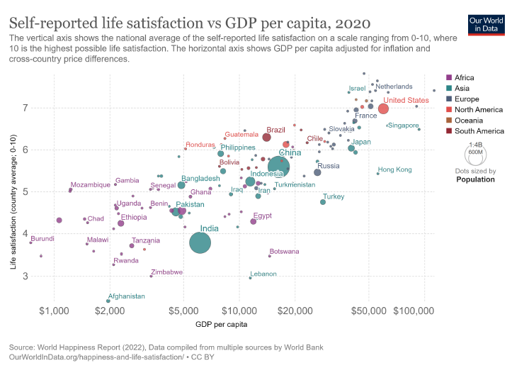
GDP ≠ measure of well-being: excludes leisure, inequality, environmental externalities, informal economy, free goods (Wikipedia). But remains the reference indicator in times of crisis to guide economic policy.
Nominal GDP vs Real GDP — Exact Formulas
🔢 GDP nominal (Teaching Notes, eq. 1.1)
\(\text{GDP}_t = \sum_{a\in A} P_{a,t} \times X_{a,t}\)
(\(A\) = set of final goods, \(P\) = price, \(X\) = quantity)
Grows if prices increase OR if the quantities increase. Model notation: \(Y_N = Y \times P\)
🔢 Real growth rate
\(g_r = \dfrac{\sum X_{a,t}\,P_{a,t-1} - \sum X_{a,t-1}\,P_{a,t-1}}{\sum X_{a,t-1}\,P_{a,t-1}}\) Key heuristic: \(g_{\text{nominal}} \approx g_{\text{real}} + \pi\) (inflation)
French method: chained indices (base renewed each year).
⚠️ Nominal/real trap
A country announces +8% nominal growth with 6% inflation → only ~2% real growth. Always deflate nominal values before comparing over time!
💡 Log decomposition (TN appendix)
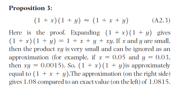
\(Y_N(t) = Y(t) \times P(t) \;\Rightarrow\; \ln Y_N = \ln Y + \ln P \;\Rightarrow\; \dfrac{\Delta Y_{N,t}}{Y_{N,t}} \approx \dfrac{\Delta Y_t}{Y_t} + \dfrac{\Delta P_t}{P_t}\)
Valid for small changes (the rule of thumb).
Limits of GDP as a measure
What GDP doesn't measure
• Domestic production (households)
• Informal and illegal economy
• Free goods (Wikipedia, open source)
• Quality of services (not just volumes)
• Inequalities and subjective well-being
• Environmental externalities
Why GDP remains useful
• Universally recognized crisis indicator
• Correlated with poverty reduction
• Guides stabilization policies
• Published frequently (quarterly + flash on D+30)
• Comparable between countries (UN-Eurostat standards)
💰 Inflation
Session 1 — Continuous increase in the general price level (Blanchard Ch.1, TN §1.3.2)
📘 Definitions
Inflation = continuous increase in the general price level. Deflation = fall continue. Disinflation = slowdown in inflation (prices are still rising, but less quickly). The price level is measured by a price index — a weighted average of the prices of all goods.
The weights \(w_i\) are the shares of each good in the representative consumption basket; \(\bar{w}_i\) are the fixed base-year weights (Laspeyres method).
📘 3 measures to know
CPI — Consumer Price Index: basket cost of a representative household, the most widely used measure. France: INSEE collects 200,000 prices monthly (99 cities, 30,000 stores). IPP/PPI : ex-factory price, excluding taxes and transport. GDP deflator: ratio \(Y_N / Y\) — price-level measure.
💡 Laspeyres CPI vs Chain-Linked CPI
Fixed-base index (Laspeyres): constant weights over several years. Chain-linked index: weight updated each year (France, euro zone). Covid problem: the 2019 weights overweighted hotels/risaurants whose prices were falling → artificially low inflation in 2020, then jump in January 2021 during the update.
📘 HICP — Zone euro
Eurostat uses the HICP (Harmonized Index of Consumer Prices). It is a weighted average of national HICPs by GDP and population. Weight 2023: Germany 27.8%, France 19.4%, Italy 16.5%, Spain 11%. Key difference with the US CPI: the HICP excludes real estate property services (only rents, 7.5% of the basket).
⚠️ Pitfalls to avoid
1. Inflation is a rate (%), not a price level. 2. Disinflation ≠ Deflation. 3. Overall inflation ≠ underlying inflation (core = excluding energy + food). The ECB targets headline inflation at 2% but monitors underlying inflation for monetary policy decisions.
🎯 Tip exam — model link
In modeling: \(P\) is a one-dimensional positive continuous variable. \(Y_N = Y \times P\). Decomposition: \(g_{n,t} = g_{r,t} + \pi_t\). This is the fundamental decomposition used throughout the course. Inflation 2022 eurozone: 10.6% (peak) → ECB raised its rates up to 4% → fell to 2% in 2026.
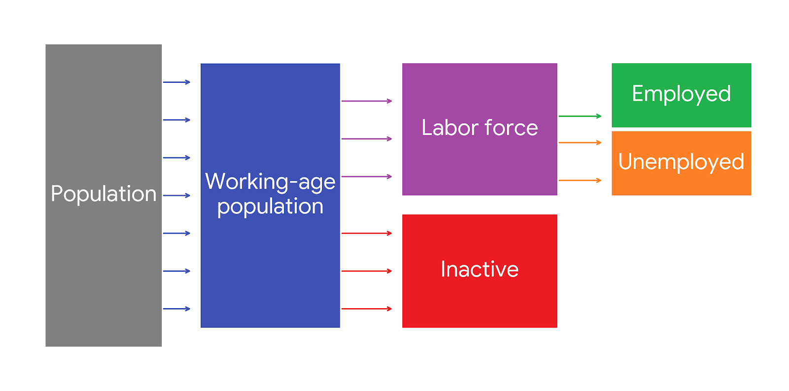
Working age population: 15–74 years (excluding children and retirees). Labor force \(L\): people who are working OR looking for work. Unemployed \(U\): unemployed, available within 2 weeks, actively looking for 4 weeks. Inactifs : students, retirees, discouraged people.
🔢 Key formulas (TN eq. 1.6–1.7)
\(L = U + E\) (labor force = unemployed + employed) \(u = U / L\) (unemployment rate) Employment rate \(= E / \text{working-age population}\) Labor productivity \(= Y / \text{hours worked}\) (chained base 2010)
💡 Definition matters
To be unemployed, you must meet the 3 conditions simultaneously: (1) unemployed, (2) available, (3) actively looking. An unaffected student = inactive, not unemployed. A discouraged worker who gives up his search → quitte the labor force population → the unemployment rate fall mechanically even without job creation!
⚠️ The trap of the unemployment rate in crisis
The unemployment rate can lower during a crisis if discouraged workers stop looking (they become inactive, fall out of the \(L\) denominator). A low rate does not necessarily mean a healthy job market. Always look at the employment rate too.
📘 Types of unemployment
Frictional unemployment: normal time between two jobs. Structural unemployment (\(u^*\)): natural rate, linked to labor market rigidities (NAIRU). It is \(u^*\) which enters the Phillips curve. Cyclical unemployment: \(u - u^*\), created by insufficient demand. This is the focus of the Keynesian model.
🎯 Encrypted benchmarks
USA Great Depression 1933: \(u = 25\%\). COVID 2020 (USA): peak at ~15%. Eurozone today: ~6%. In the Keynesian model, unemployment is only caused by insufficient demand (companies do not have enough orders to employ all available labor).
🏦 Interest Rates
Session 3 — The price of money and engine of monetary policy
📘 Real vs Nominal
Nominal rate (\(i\)): The stated rate on a loan or bond. Real rate (\(r\)): Nominal rate minus expected inflation: \(r = i - \pi^e\)
The real rate is what matters for investment decisions.
🧠 Short vs Long rates
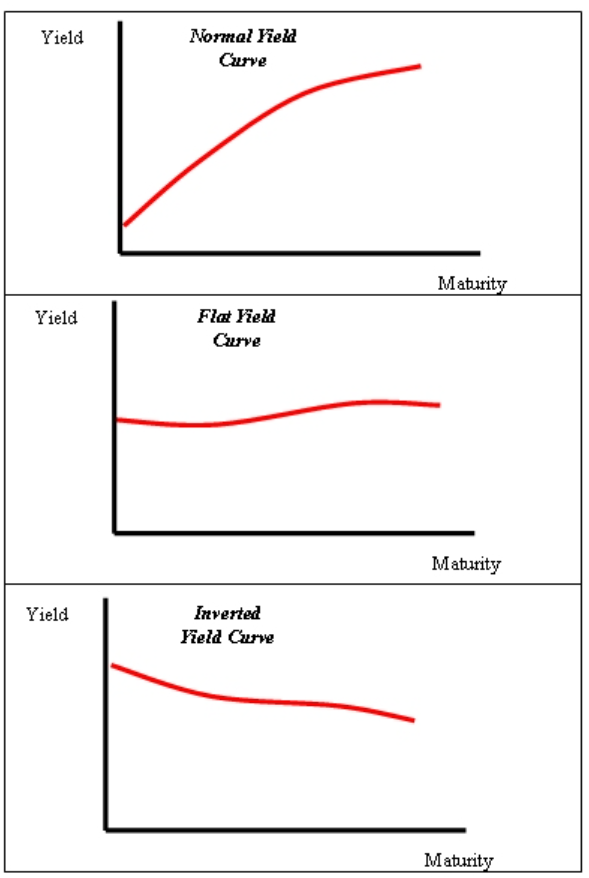
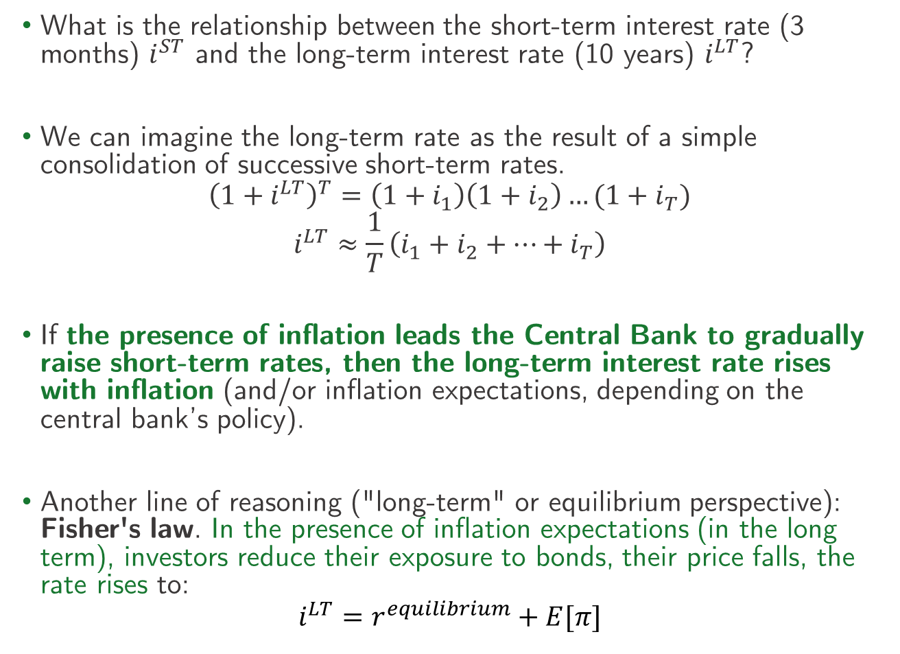
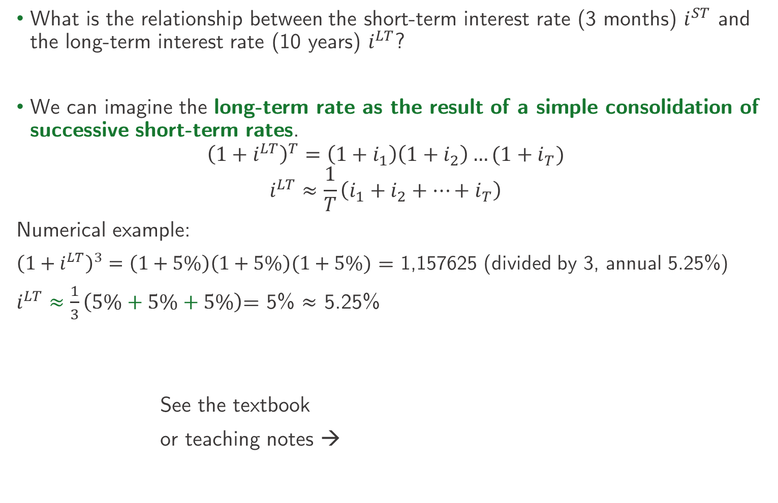
Short-term rates are set by central banks (Fed, ECB). Long-term rates are determined by bond markets and reflect expectations of future short rates + a term premium. When markets expect inflation to fall, the yield curve can invert (short > long).
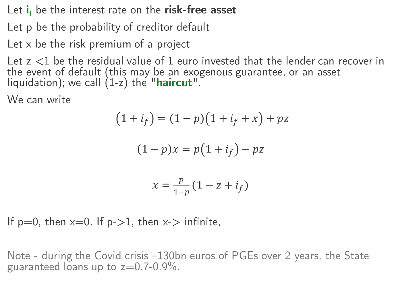
📘 Risk premium
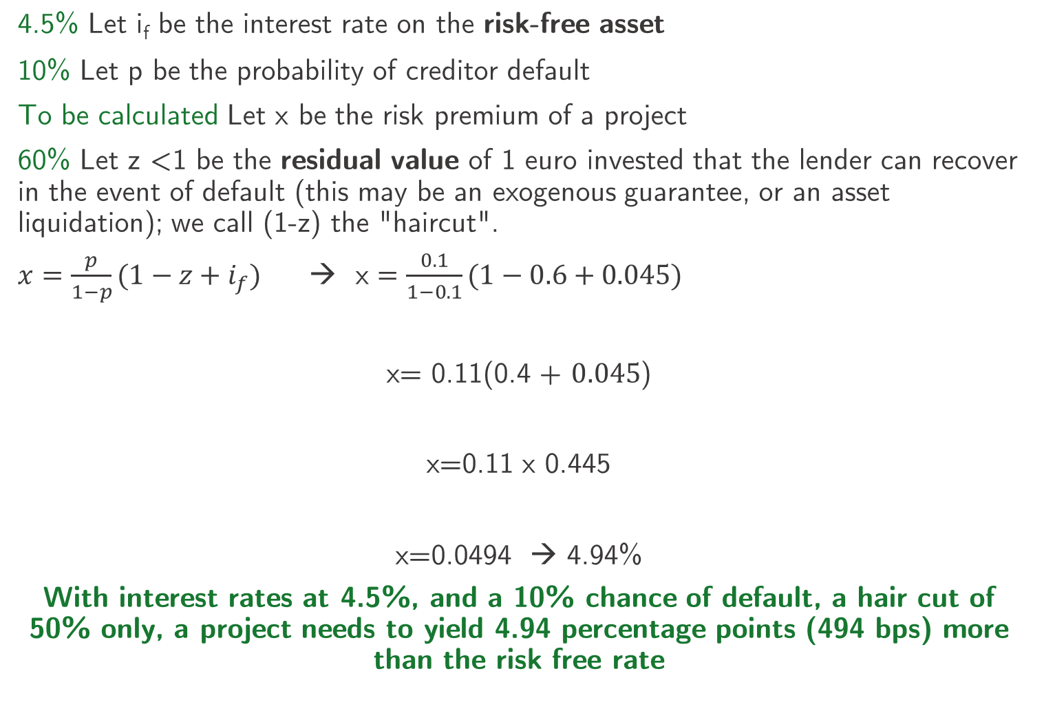
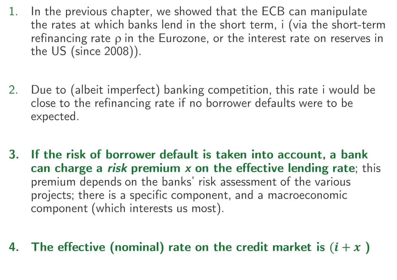
A risky borrower must pay a risk premium \(x\) above the risk-free rate. It compensates lenders for the probability of default (\(p\)) and the loss given default (\(1-z\), where \(z\) is residual value).
Current context: Fed rate ~3.50-3.75%, ECB ~2%. Be ready to discuss why rates differ and how they affect investment, debt sustainability (\(i\) vs \(g\)), and exchange rates.
⚙️ The Keynesian Model
Session 2 — Demand determines production in crisis (Blanchard Ch.2, TN §2.1–2.5)
📘 Central idea (Keynes, 1936)
During periods of demand crisis, the economy operates below full employment (\(Y < Y^*\)). Prices are rigid, supply adapts to demand. Demand determines production. Equilibrium condition: \(Y = Y^d\). The Great Depression revealed that an economy can remain permanently stuck in imbalance.
📘 6 simplifying assumptions
H1 : Economy below full employment (\(Y < Y^*\)) H2 : Rigid prices in the short term (constant \(P\), horizontal supply) H3 : Companies produce what demand requires H4 : Supply = Income (\(Y^s = Y\)) — €1 of sale = €1 of income H5 : Exogenous interest rate (relaxed in session 3) H6 : Closed economy: \(X = IM = 0\) (released sessions 8–10)
🔢 Aggregate demand and balance
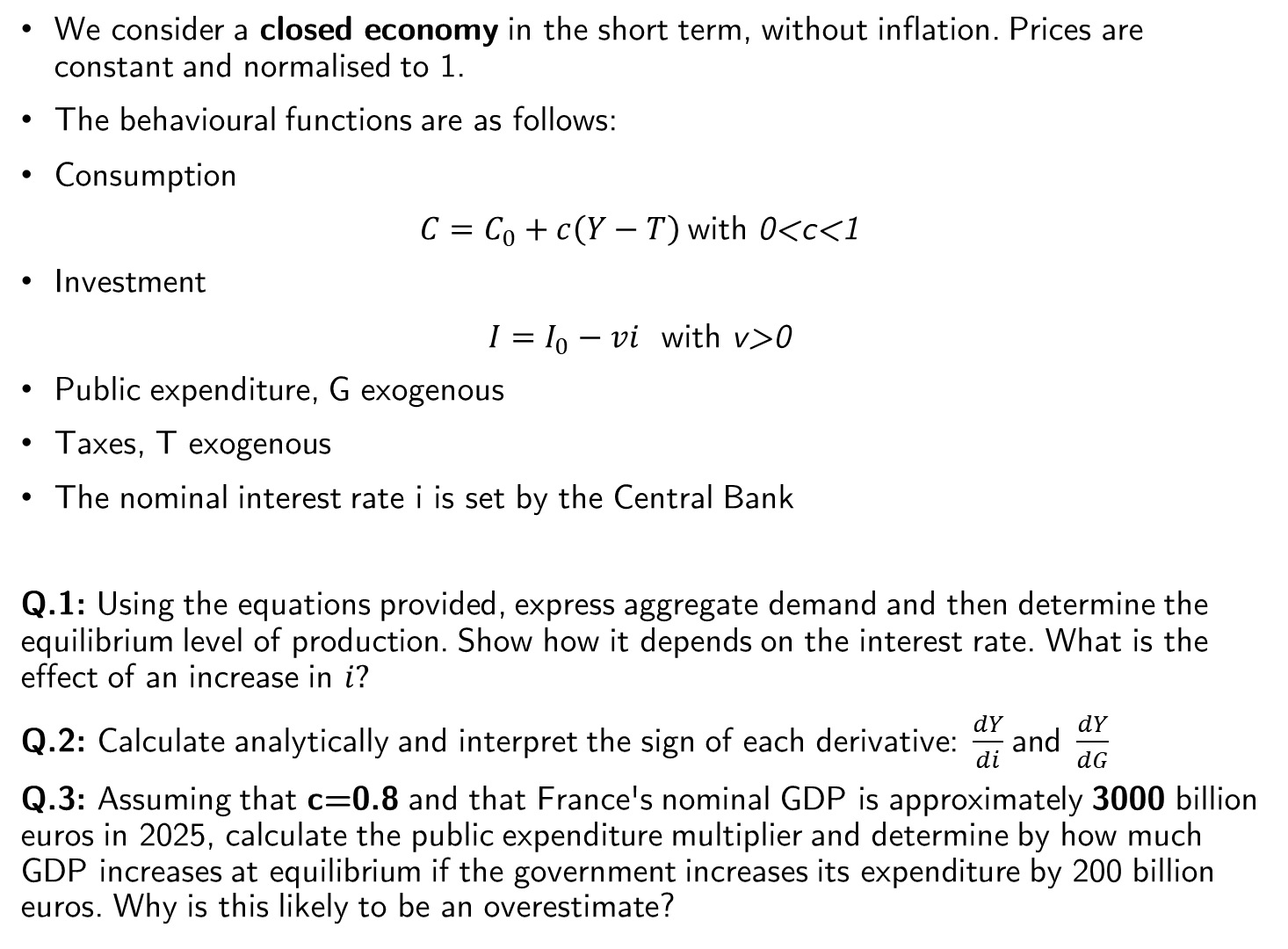
\(Y^d = C + I + G\) (closed eco)
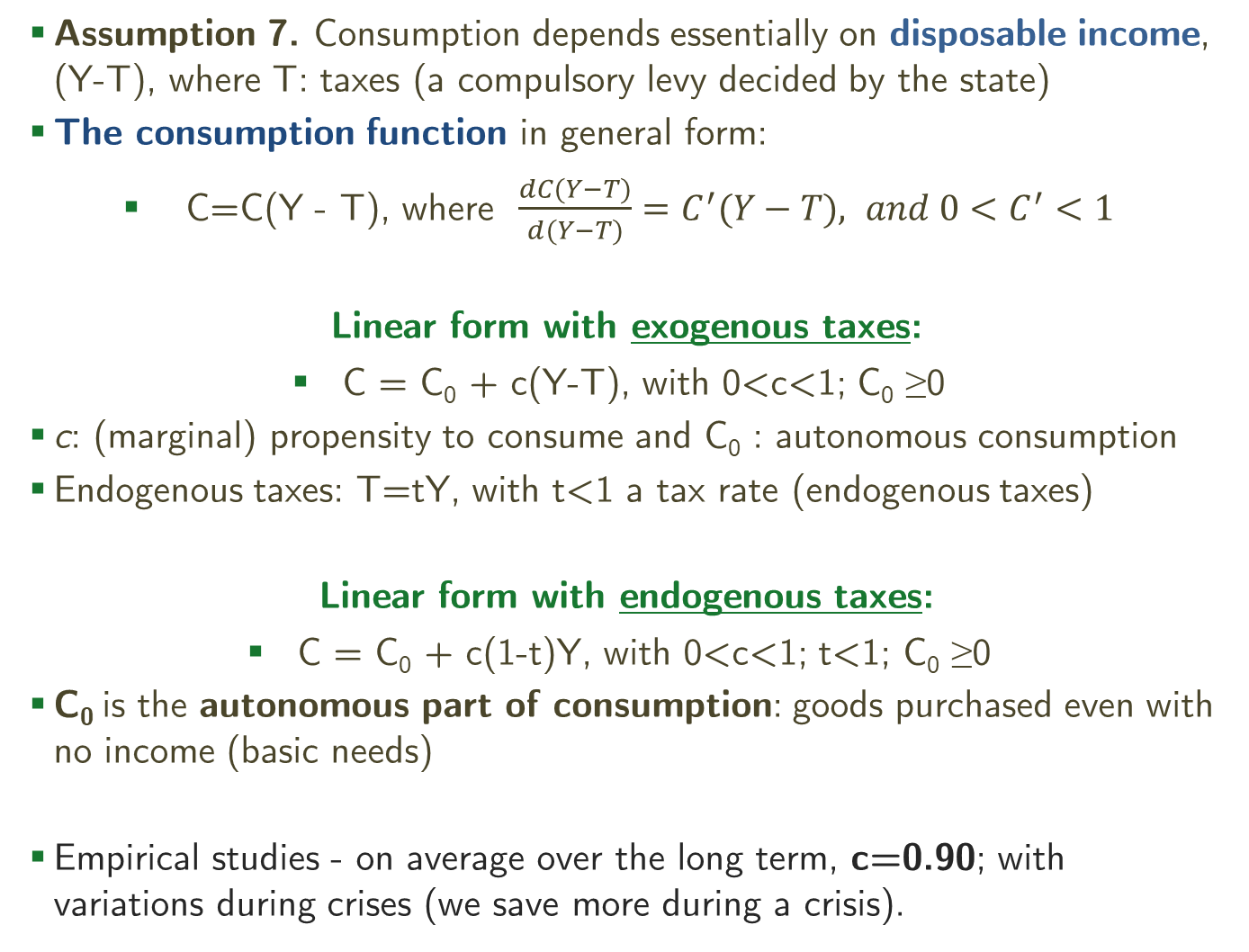
\(C = C_0 + c(Y - T)\) with \(0 < c < 1\) Balance: \(Y^* = \frac{1}{1-c}(C_0 - cT + I + G)\) IS identity: \(S + (T - G) = I\) (private + public savings = investment)
⚠️ Demand crisis ≠ supply crisis
The Keynesian model applies only for demand crises (Great Depression, GFC 2008, Euro crisis 2010). Supply shocks (oil 1973/79, Ukraine war 2022, Covid on the supply side) require different tools. Classic error: applying a stimulus policy to a supply shock.
💡 Classification of seizures
Demand crises: Great Depression 1929, GFC 2007-09, Euro Crisis 2010-12 Supply: Oil shocks 1973/1979, Ukraine war (energy 2022) Mixed: COVID-19 (simultaneous supply + demand collapse)
Paradox of thrift (Teaching Notes, Ex. 1)
💡 The paradox of frugality
If all households decide to save more (\(c\downarrow\)), aggregate demand falls → equilibrium \(Y^*\) falls → income decreases → total savings do not change (or decrease)! What is individually rational (saving) becomes collectively harmful. Formally: \(Y^* = \frac{1}{1-c}(\dots)\) → if \(c\downarrow\) then \(\frac{1}{1-c}\downarrow\) therefore \(Y^*\downarrow\). This is Keynes' "paradox of thrift".
🔄 Tax Multipliers
Session 2 — How fiscal policy amplifies demand (TN §2.5)
🔢 Balance — exogenous taxes T
\(Y^* = \frac{1}{1-c}\,(C_0 - cT + I + G)\) Spending multiplier: \(dY/dG = 1/(1-c)\) Tax multiplier: \(dY/dT = -c/(1-c)\) A tax cut is always less powerful than direct spending: \(\left|-c/(1-c)\right| < 1/(1-c)\)
💡 Multiplier Mechanism
If \(c = 0.8\) and \(dG = 100\) :
Round 1: \(+100\) demand → \(+100\) income
Round 2: \(+80\) consumption (\(0.8\times100\)) → \(+80\) income
Round 3: \(+64\) (\(0.8\times80\)) → …
Total: \(100 \times \frac{1}{1-0.8} =\) 500
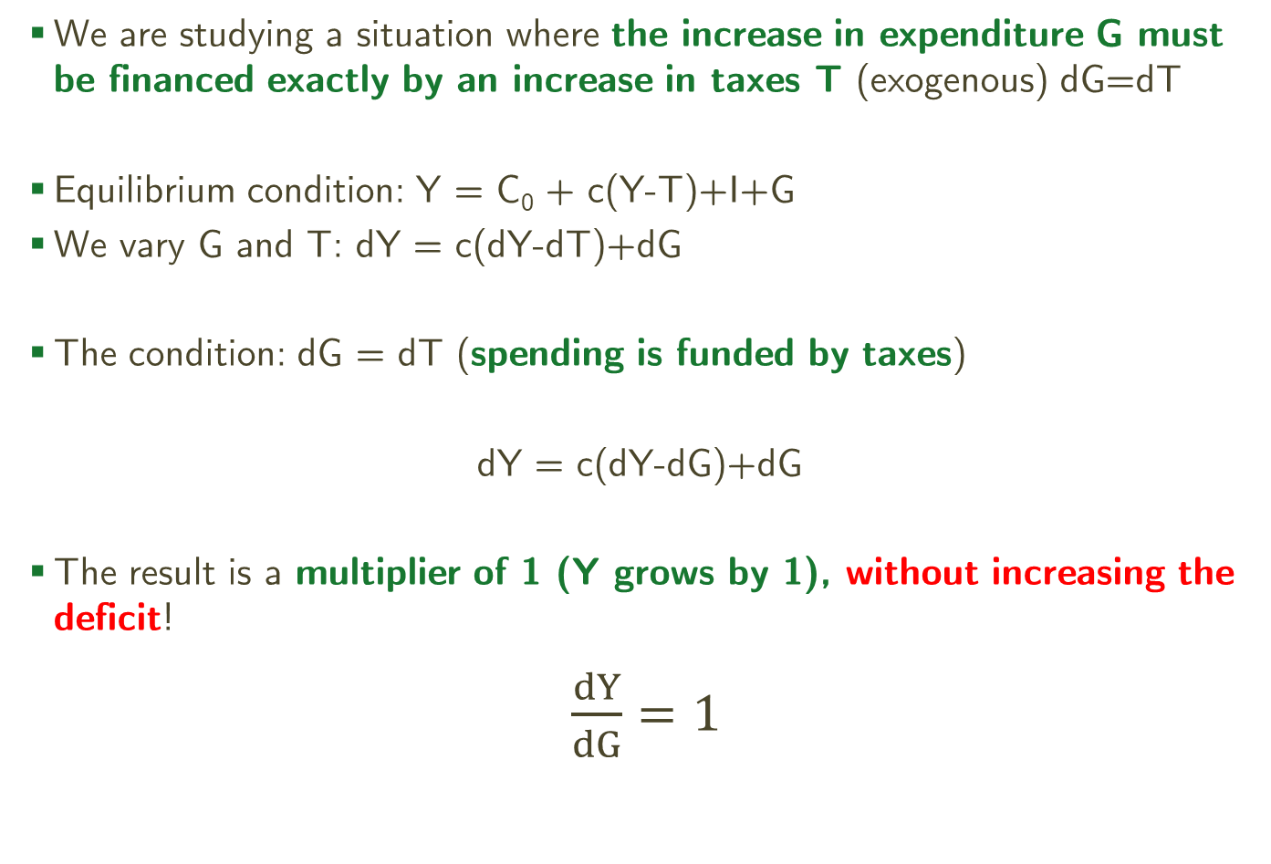
🎯 Balanced budget theorem (TN Ex. 2)
If \(dG = dT\) (simultaneous expenditure + tax financing):
\(dY = dG \times \frac{1}{1-c} + dT \times \left(\frac{-c}{1-c}\right) = dG \times 1\) Multiplier = 1. The economy grows by exactly \(dG\), even at a constant deficit. Why? The initial net shock is \(dG - c\,dT = dG(1-c) > 0\).
🔢 Equilibrium — endogenous taxes T = tY
\(Y^* = \frac{1}{1-c(1-t)}\,(C_0 + I + G)\)
Multiplier \(= \frac{1}{1-c(1-t)}\) — smaller than with exogenous taxes. Each round of spending generates income, but a fraction \(t\) is taxed before consumption.
💡 Why smaller?
With \(T = tY\), each euro of additional income generates only \(c(1-t)Y\) of additional consumption (instead of \(cY\)). Taxes "absorb" a portion of each round. Automatic stabilizer integrated into the tax structure.
⚠️ Theory vs reality
With \(c = 0.9\) and \(t = 0.1\) → multiplier ≈ 5. In practice, the estimated multipliers are 1–3 (higher in recession, lower in expansion). Import gap, interest rate effects and expectations.
📘 Automatic stabilizers (TN Ex. 4)
Integrated mechanisms that cushion the cycle without political decision. Examples: progressive income tax (taxes collect more in booms and less in crises), unemployment benefits. Result: the effective multiplier is \(\dfrac{1}{1-c+\delta}\) with \(\delta\) = unemployment replacement rate. The larger \(\delta\), the more the fluctuations are damped.
💡 Mechanism (TN Ex. 4 — unemployment)
In recession: employment \(N\downarrow\) → unemployment \(U\uparrow\) → unemployment benefits \(UB\uparrow\) → consumption of the unemployed maintained → cushioning of the fall in \(Y\). In boom: opposite. The unemployed consume 100% of their allowance (\(c_{\text{unemployed}} = 1 > c_{\text{employed}}\)).
🔢 Multiplier with stabilizer (TN eq. 2.39)
\(Y^* = \dfrac{1}{1-c+\delta}\,(I + G - cT + \delta Y^*)\)
\(dY/dI = \dfrac{1}{1-c+\delta} < \dfrac{1}{1-c}\)
The higher \(\delta\) (replacement rate) → lower multiplier → more stable economy.
Inequalities and multiplier (TN Ex. 3)
💡 The paradox of inequality in Keynesian economics
If poor households consume 100% of their income (\(c_{\text{poor}} = 1\)) and the rich only \(c < 1\): a redistribution from the rich to the poor (\(dT = dF > 0\)) has a multiplier of \(1/a > 1\) — superior to the balanced budget theorem. Inequality dampens demand because the rich save more (link with "trickle-up economy" — The Economist, Feb. 2020).
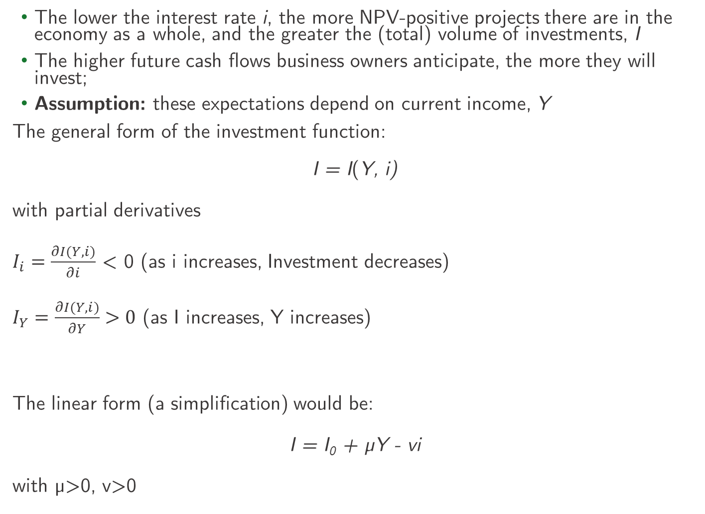
\(I = I_0 + \mu Y - v i\) \(I_0\) : independent investment \(\mu Y\) : accelerator effect (investments increase with activity) \(-vi\) : investment falls when rates rise (\(v\) = sensitivity)
Micro foundation: a company invests if \(\text{NPV} > 0\). The higher \(i\) is → more projects with \(\text{NPV} < 0\) → less investment.
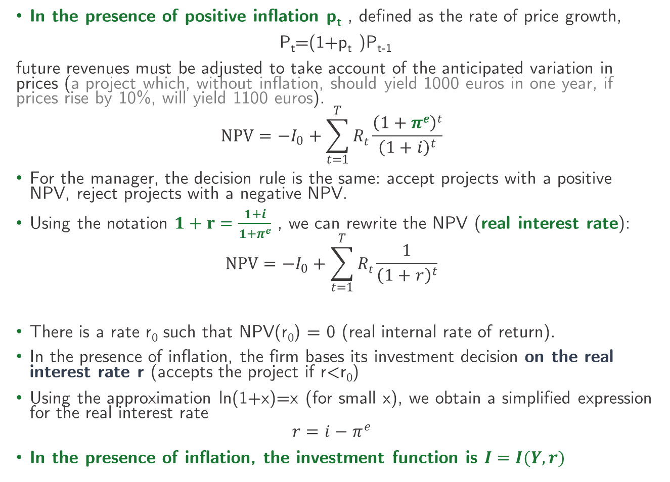
💡 Logique NPV (TN eq. 3.1)
\(\text{NPV} = -I_0 + \sum R_t/(1+i)^t\). There exists a critical rate \(\hat{\imath}\) (marginal rate of return) such that \(\text{NPV}(\hat{\imath}) = 0\). If \(i < \hat{\imath}\) → \(\text{NPV} > 0\) → profitable project. Each project has its own critical rate. Aggregate investment = sum of costs of all positive NPV projects.
🔢 IS curve — derivation
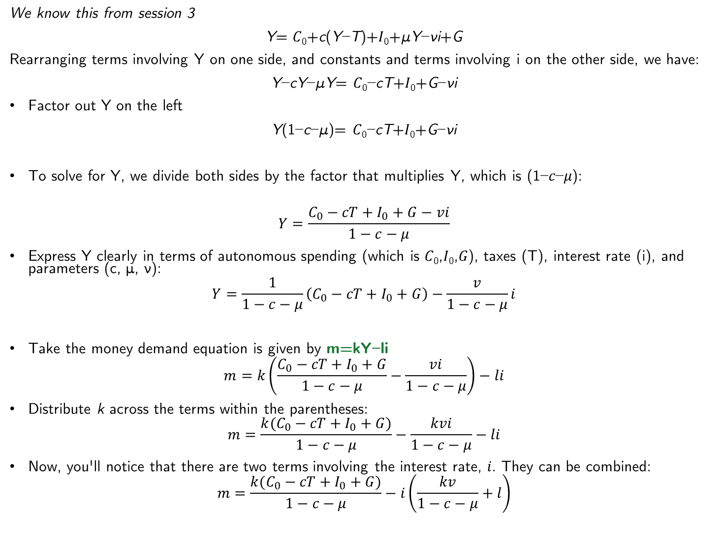
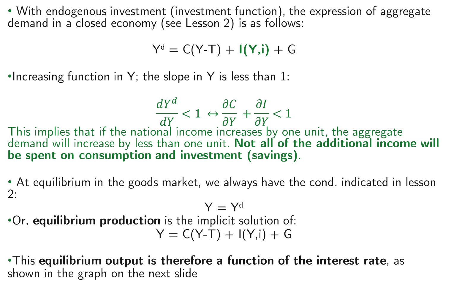
Substituting I(Y,i) into Y = C + I(Y,i) + G and solving: \(Y^* = \frac{1}{1-c(1-t)-\mu}\,(C_0 + I_0 - vi + G)\)
The IS curve represents all the pairs (Y, i) where the goods market is in equilibrium. It is decreasing: \(i\downarrow \to I\uparrow \to Y\uparrow\).
💡 Shifts of the IS curve
\(G\uparrow\) → IS moves to right (higher demand) \(T\uparrow\) → IS moves to left (less demand)
The magnitude of the shift = dG × tax multiplier. Slope of IS: depends on \(v\) (sensitivity of \(I\) to the rate) and the multiplier. More vertical IS = less rate-sensitive investment.
📘 Risk premium (TN §3.2.1)
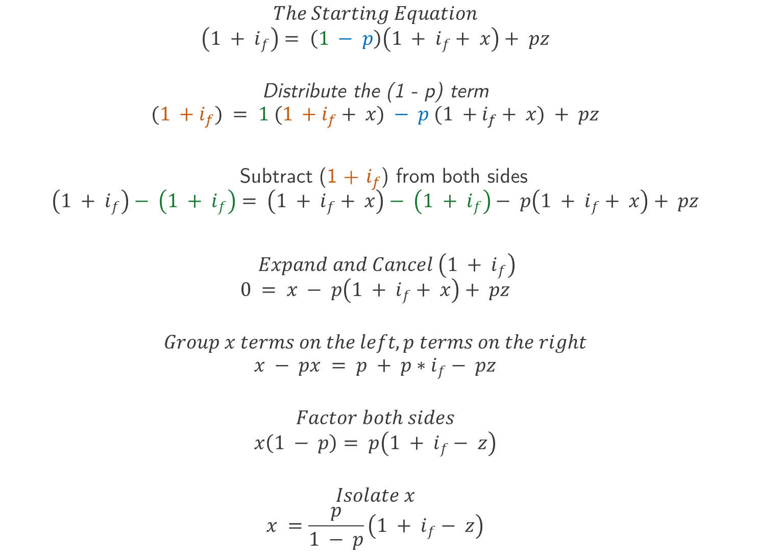
A risky borrower pays: \(i = i_{\text{free}} + \psi\). The risk premium \(\psi\) depends on the probability of default \(p\) and the residual value \(z\):
\((1+i_f) = (1-p)(1+i_f+\psi) + p\,z\) → \(\psi = p(1-z+i_f)/(1-p)\)
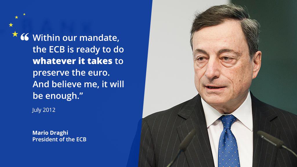
Application 2012: Greece, haircut 53.5% → huge risk premium. Draghi + OMT → collapsed risk premium.
🔢 Real rate (Fisher, TN §3.2.3)
\(r = i - \pi^e\) (nominal rate − expected inflation)
Long-term rate: \(i_{LT} = r_{eq} + E[\pi]\)
This is the real rate that matters for investment decisions, not the nominal rate.
Standard exercise (TN §3.1.1) — Investment projects
🎯 Classic exercise for the exam
3 projects A, B, C with cost and cash flows over several years. Calculate the marginal rate of return î (rate for which NPV = 0). Build the staircase investment function : \(I(i) = 410\) if \(i < 7\%\); 200 if \(7\% \le i < 10\%\); 100 if \(10\% \le i < 16\%\); 0 if \(i \ge 16\%\). See the Practice section for the complete exercise.
📉 Dynamics of Public Debt
Session 3 — When does debt become unsustainable? (Blanchard AEA 2019, TN §2.6–2.7)
🔢 Debt dynamics (TN eq. 2.33–2.34)
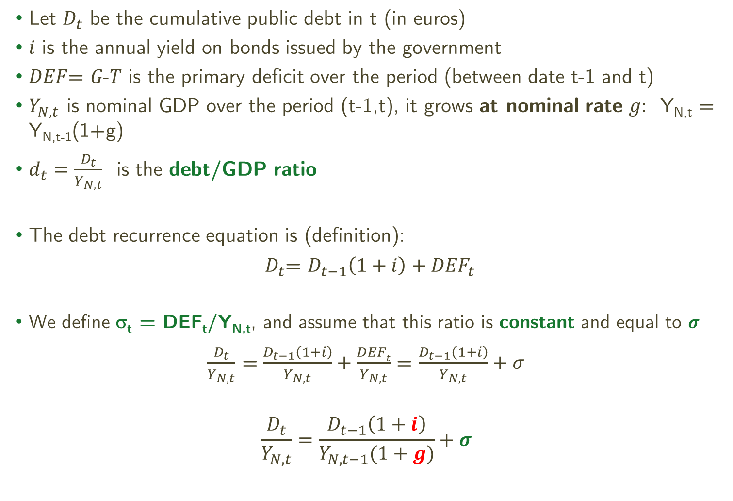
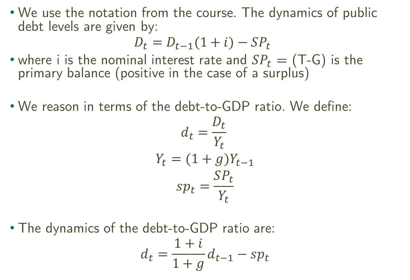
\(D_t = D_{t-1}(1+i) + DEF_t\) (in absolute value)
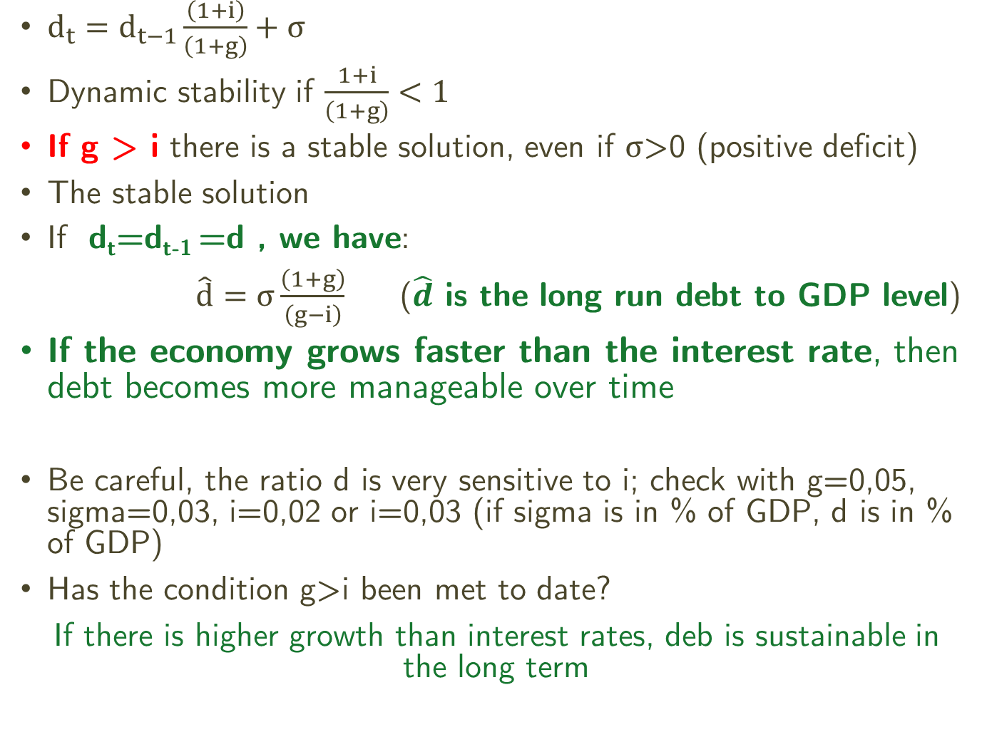
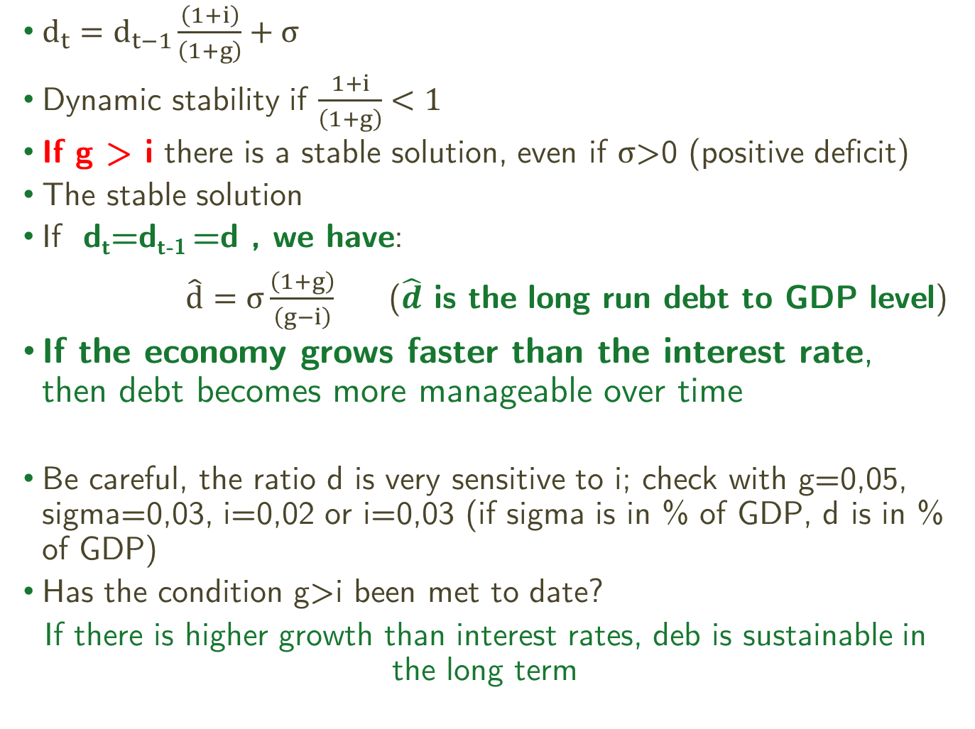
A debt/GDP ratio (\(d_t = D_t/Y^e_t\)): \(d_t = \dfrac{1+i}{1+g_n}\,d_{t-1} + \sigma\)
where \(\sigma = DEF/Y\) = deficit/GDP ratio (fiscal rule)
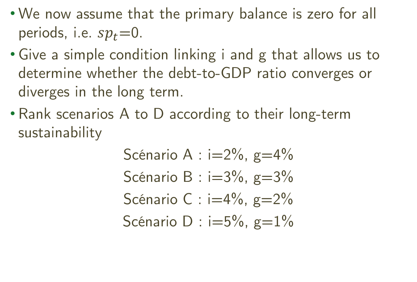
💡 The rule i < g (Blanchard, 2019)
Dynamic stability condition: \(\dfrac{1+i}{1+g_n} < 1 \iff i < g_n\)
If \(i < g\) (nominal growth rate) → the debt converges even with deficits.
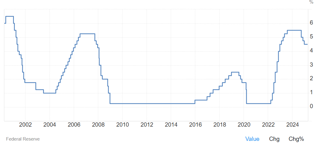
If \(i > g\) → the debt diverges (snowball effect). In 2019: condition verified → Blanchard minimized the danger. In 2022–24: i rises, g stagnates → reversed condition in many countries.
🔢 Value steady-state (TN eq. 2.36)
If \(i < g\), \(d\) converges to: \(\hat{d} = \dfrac{\sigma(1+g_n)}{g_n-i}\)
Ex: \(\sigma = 3\%\), \(g = 5\%\), \(i = 2\%\) → \(\hat{d} = 0.03 \times 1.05/0.03 =\) 105% of GDP
📘 Contexte current (2026)
France: deficit ≈ 6% GDP, debt ≈ 115% GDP, ECB rate ≈ 2%, growth ≈ 0.9%. Condition: \(i\) (2%) > \(g\) (0.9%) → the debt is not stable with these parameters. This is why market pressure is exerted on French sovereign rates. Cf. Liz Truss UK 2022: irresponsible tax announcement → bond markets punished her in 49 days.
⚠️ The real debt trap
Looking only at the deficit is insufficient. A country with a 6% deficit but 5% nominal growth (\(g > i\)) may have a more sustainable debt than a country with a 2% deficit, 0% growth and 3% interest rate. THE ratios and the dynamics matter, not absolute values.
🎯 Exam application (TN Ex. 7)
\(\sigma = 3\%\), \(g_n = 5\%\), \(i = 2\%\) → \(i < g\) → stable. \(\hat{d} = 1.05/0.03 = 105\%\). If \(g\) increases by 1pp → \(\hat{d} = 1.06/0.04 = 79.5\%\). Knowing how to calculate this trajectory quickly is fundamental for the exam.
Stability Pact & Euro Zone Crisis
1999
Stability and Growth Pact (PSC)
Maastricht rules: deficit < 3% GDP, debt < 60% GDP. Violated by France and Germany since 2005 without sanction — damaged credibility.
2010
Sovereign debt crisis — Greece, Ireland, Portugal, Spain
Greece: 130% debt/GDP, downgraded to "junk". Troika (IMF/ECB/CE) → €110 billion loan + 53.5% haircut on private debt in 2012.
2012
OMT — "Whatever it takes" (Draghi)
OMT = unlimited conditional redemptions. Never used. His single announcement was enough to crush sovereign spreads and put an end to the crisis. Historic moment.
2025
ReARM Europe — €800 milliards
Response to the Trump strategic pivot. Countries spending +1.5% GDP on defense exempt from the 3% rule. Germany: €1 trillion plan over 10 years.
🧮 All Key Formulas
Your formula sheet for exam day
📐Key formulas in math notation (KaTeX)▼
Typographic rendering of the major formulas. If nothing shows up, KaTeX is still loading — refresh the page.
Fiscal multiplier (endogenous tax)
$$\frac{dY}{dG} = \frac{1}{1 - c(1-t)}$$
Linear IS curve
$$Y^* = \frac{1}{1 - c - \mu}\big[C_0 - cT + I_0 + G - vi\big]$$
Golden rule: in the exam, identify the assumptions first (T endogenous or exogenous? I endogenous or exogenous? open economy?) BEFORE picking the formula. Wrong variant = direct loss of points.
The 4 interest rates — never confuse them
Symbol
Name
Definition
Used for
\(i\)
Nominal rate
Posted rate, what the CB sets
LM, UIP, bond pricing
\(r = i - \pi^e\)
Expected real rate
True borrowing cost, inflation-adjusted
Investment decisions (NPV, IS)
\(r^*\)
Natural rate (Wicksell)
Real rate consistent with Y=Y* and stable π
Reference for Taylor rule, medium-term
\(i + \psi\)
Risk-adjusted rate
i + default/liquidity premium ψ
Effective borrowing cost for firms/households
Frequent trap: investment decisions use \(r = i - \pi^e\), NOT \(i\) alone. And \(r^*\) is never directly observable — the CB estimates it.
IS, LM, PC — what shifts vs. what moves along?
IS curve (Y, r) Shifts with: \(\Delta G, \Delta T, \Delta c_0, \Delta\psi, \Delta X_0, \Delta\pi^e\). Moves along with: \(\Delta r\) only (CB changes \(i\), \(\pi^e\) fixed).
LM curve (Y, i) Shifts with: ΔM, ΔP (real M), Δ autonomous money demand. Moves along with: ΔY only.
PC curve (π, u) Shifts with: \(\Delta\pi^e, \Delta m, \Delta z, \Delta\sigma\) (supply shocks). Moves along with: \(\Delta u\) only (demand changes).
Keynesian cross \((Y,Y^d)\) Shifts with: \(\Delta C_0,\Delta I_0,\Delta G,\Delta T,\Delta X_0,\Delta IM_0\). Moves along with: \(\Delta Y\) because induced consumption changes along \(Y^d=C_0+c(Y-T)+I+G\).
WS-PS model \((u,W/P)\) Shifts with: \(\Delta m,\Delta\sigma,\Delta z,\Delta A,\Delta A^e\). Moves along is not the main story: equilibrium is where WS and PS intersect; shocks move one curve and therefore \(u^*\).
Interactive shift guide
Choose a model and a shock to see whether the curve shifts or the equilibrium moves along it.
🔤 Variables Glossary
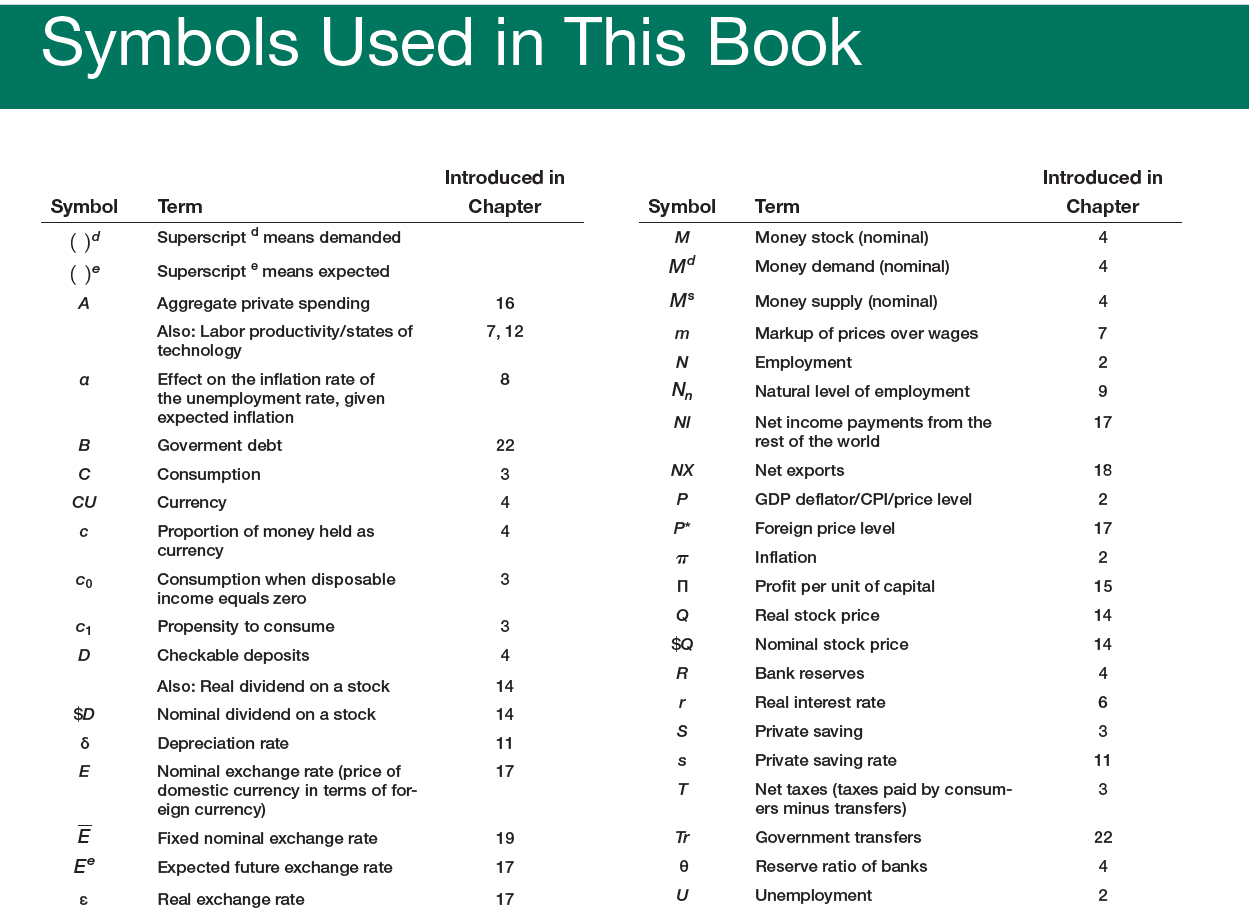
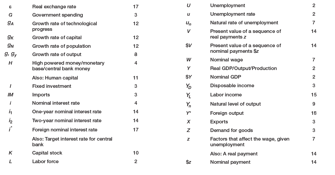
All symbols used in the course — sorted by category
SymbolNameDescription
\(Y\)Real GDP / Output / IncomeThe total value of final goods & services produced, at constant prices. In the Keynesian model, \(Y\) also represents aggregate income (Assumption 4: \(Y^s = Y\)).
\(Y_N\)Nominal GDPGDP valued at current prices. \(Y_N = Y \times P\). Grows with both real output and inflation.
\(Y^*\)Equilibrium outputThe level of output where supply equals demand (\(Y^s = Y^d\)). The solution to the Keynesian model.
\(Y_{FE}\)Full employment outputMaximum output when all resources are fully employed. In a demand crisis, \(Y < Y_{FE}\) (the economy operates below potential).
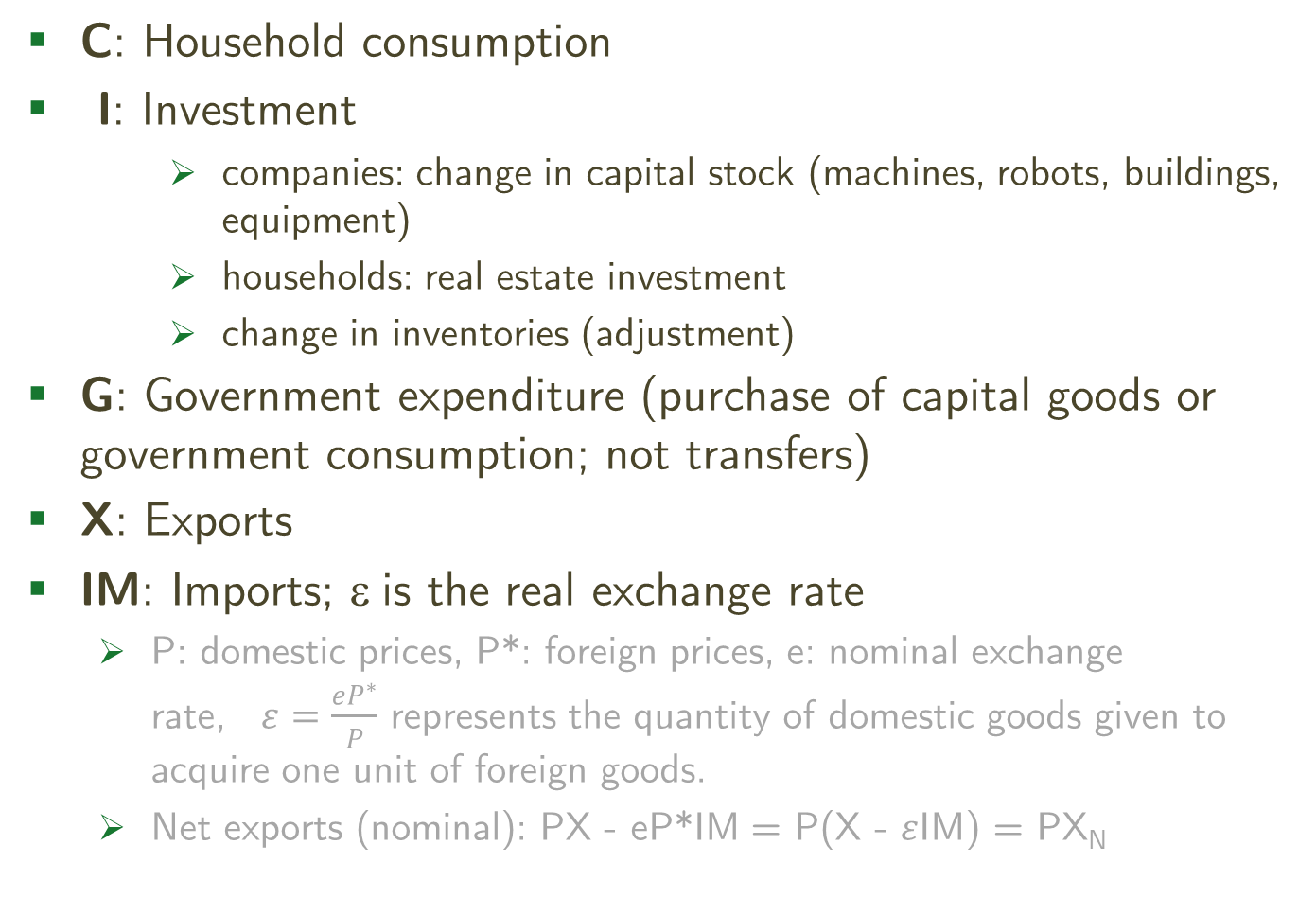
\(Y^d\)Aggregate demandTotal demand for goods & services: \(Y^d = C + I + G + (X - IM)\). Determines output in the Keynesian model.
\(Y^s\)Aggregate supplyTotal production. Under Keynesian assumptions, supply adjusts to demand (horizontal supply curve). \(Y^s = Y\).
\(g\)GDP growth rateReal GDP growth rate: \(g = \Delta Y / Y\). Critical in debt dynamics (sustainability condition: \(i < g\)).
\(P\)General price levelA one-dimensional, continuous, positive variable representing the price index (e.g. CPI). Normalized to \(P = 1\) in the short-term Keynesian model.
SymbolNameDescription
\(C\)ConsumptionHousehold spending on goods & services. \(C = C_0 + c(Y - T)\) or \(C = C_0 + c(1-t)Y\). The largest component of GDP.
\(C_0\)Autonomous consumptionThe part of consumption independent of income (basic necessities, etc.). Even with zero income, \(C_0 > 0\).
\(I\)InvestmentBusiness spending on capital goods (machines, buildings). \(I = I_0 + \mu Y - v\,i\). Falls when interest rates rise.
\(I_0\)Autonomous investmentThe part of investment not influenced by income or interest rates (e.g. government infrastructure projects, strategic investments).
\(G\)Government spendingPublic expenditure on goods & services. Exogenous policy variable. Increasing \(G\) is fiscal stimulus (shifts IS right).
\(T\)Taxes (exogenous)Total tax revenue as a fixed amount (lump-sum). Used in the exogenous tax model. Disposable income \(= Y - T\).
\(X\)ExportsGoods & services sold to the rest of the world. Set to 0 in the closed-economy model (Assumption 6).
\(IM\)ImportsGoods & services bought from abroad. Set to 0 in the closed-economy model.
\(S\)SavingsIncome not consumed and not taxed: \(S = Y - C - T\). Appears in the IS identity: \(S + (T - G) = I\).
SymbolNameDescription
\(c\)Marginal propensity to consumeFraction of each additional euro of disposable income that is consumed. \(0 < c < 1\). Typical values: 0.8–0.9. Drives the multiplier.
\(t\)Tax rate (endogenous)Tax as a proportion of income. \(\text{Taxes} = tY\). Endogenous model: taxes vary automatically with income (automatic stabilizer). Typical value for France: ~0.45.
\(\mu\)Income sensitivity of investmentMeasures how much investment changes per unit change in national income (accelerator effect). Appears in \(I = I_0 + \mu Y - v\,i\).
\(v\)Interest rate sensitivity of investmentHow much investment falls when interest rate rises by 1 point (100 bps). Higher \(v\) → steeper investment function, flatter IS curve.
\(\frac{1}{1-c}\)Spending multiplier (exo T)Total change in GDP per unit change in \(G\), with fixed lump-sum taxes. If \(c = 0.8\), multiplier \(= 5\).
\(\frac{1}{1-c(1-t)}\)Spending multiplier (endo t)Total change in GDP per unit change in \(G\), with proportional taxes. Always smaller than \(\frac{1}{1-c}\) because taxes absorb part of the income increase.
\(\frac{-c}{1-c}\)Tax multiplier (exo T)Total change in GDP per unit increase in lump-sum taxes \(T\). Negative (higher taxes reduce GDP). Smaller in abs. value than spending multiplier.
SymbolNameDescription
\(i\)Nominal interest rateThe stated rate on a loan or bond. Set by central banks (short-term) or bond markets (long-term). Key policy variable.
\(r\)Real interest rateNominal rate minus expected inflation: \(r = i - \pi^e\). What matters for investment and savings decisions.
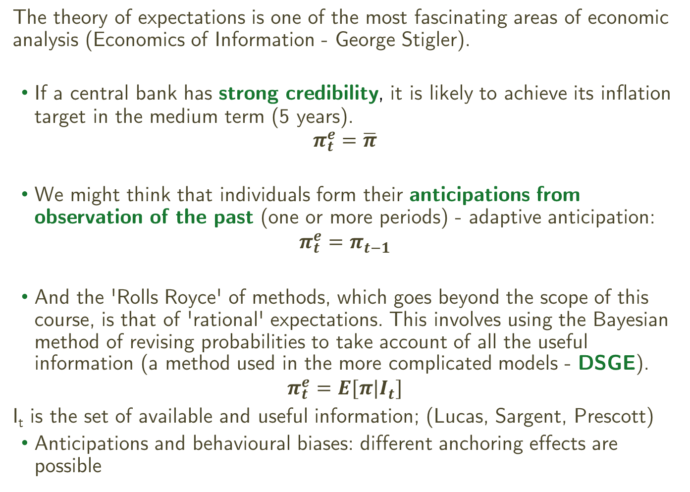
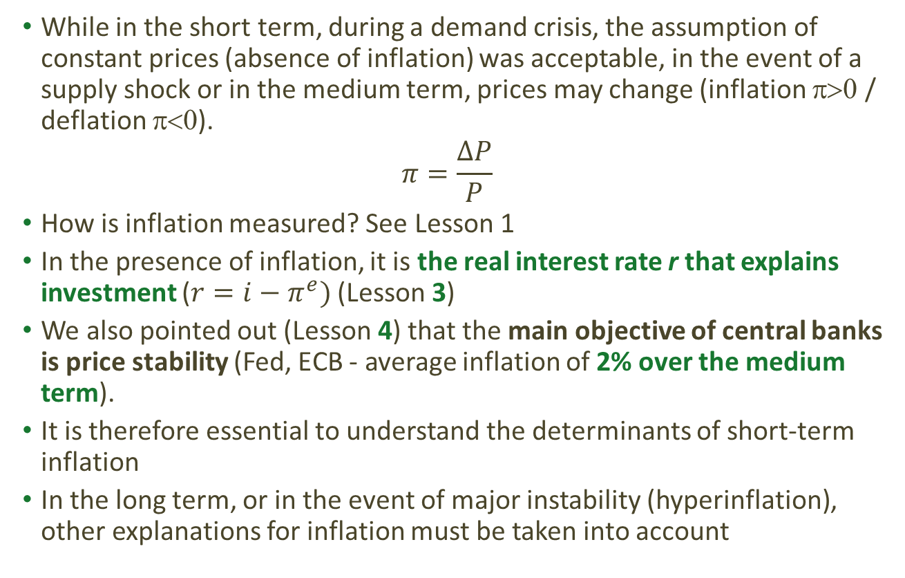
\(\pi / \pi^e\)Inflation / Expected inflation\(\displaystyle \pi = \dfrac{\Delta P}{P}\) (rate of change of the general price level). \(\pi^e\) is the market's expectation of future inflation.
\(i_f\)Risk-free interest rateThe rate on a default-free asset (e.g. government bonds of a safe country). Baseline for computing risk premiums.
\(x\)Risk premiumExtra return demanded by lenders above \(i_f\) to compensate for default risk. Depends on default probability (\(p\)) and loss given default (\(1-z\)).
\(p\)Default probabilityProbability that the borrower fails to repay. Increases the risk premium.
\(z\)Residual valueFraction of the loan recovered in case of default (\(0 \le z < 1\)). Higher \(z\) → lower loss → lower risk premium.
\(D\)Public debt (stock)Total accumulated government debt. \(D/Y\) = debt-to-GDP ratio, the standard measure of fiscal sustainability.
\(\text{Def}\)Budget deficit\(\text{Deficit} = G - T\) (or \(G - tY\)). When \(G > T\), the government borrows. The deficit adds to the debt stock each year.
\(\text{NPV}\)Net Present ValuePresent value of future cash flows minus initial cost. Decision rule: invest if \(\text{NPV} > 0\). \(\text{NPV}\) falls when \(i\) rises.
SymbolNameDescription
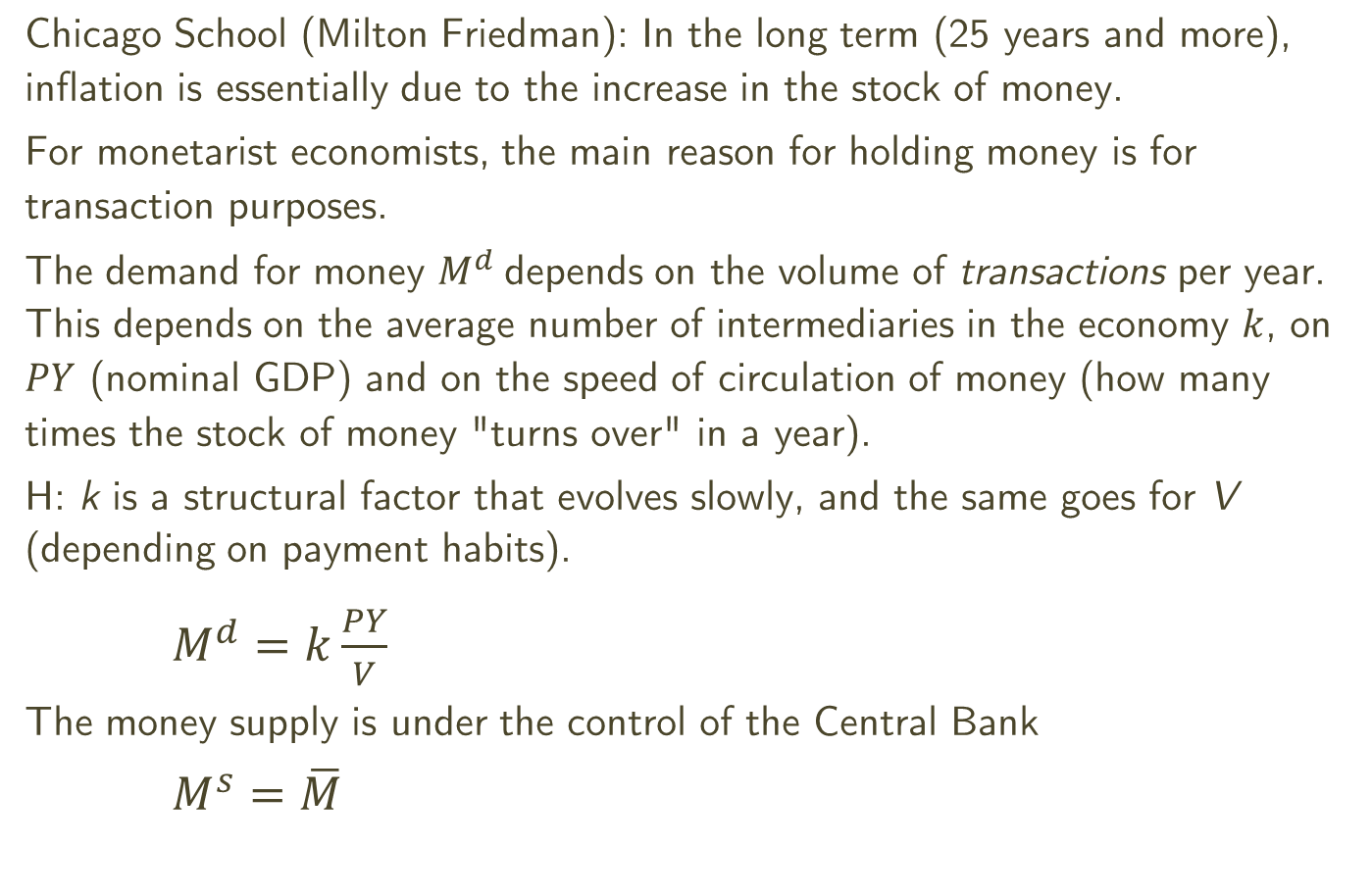
\(M / \bar{M}\)Money supplyTotal stock of money = banknotes + bank deposits. \(\bar{M}\) meanss CB-controlled supply.
\(M^d\)Money demandDesired money holdings. Depends positively on \(Y\), negatively on \(i\). Linear form: \(M^d = k\,Y_{\text{EUR}} - l\,i\).
\(m\)Real money balances\(\displaystyle m = \dfrac{M}{P}\). Real purchasing power of the money stock.
\(k,\,l\)Money demand parameters\(k\) = income sensitivity (higher \(Y\) → more \(M^d\)). \(l\) = interest sensitivity (higher \(i\) → less \(M^d\)).
\(L(i)\)Liquidity preferenceDecreasing function of \(i\). In multiplicative form \(M^d = Y_{\text{EUR}}\,L(i)\).
\(P_B\)Bond priceInversely related to \(i\). For a 1-year zero-coupon bond with face value \(F\): \(\displaystyle P_B = \dfrac{F}{1+i}\).
\(u\)Unemployment rateShare of the labor force without a job: \(u = \dfrac{L - N}{L}\). The WS curve is decreasing in \(u\) (more unemployment → weaker worker bargaining power → lower wages).
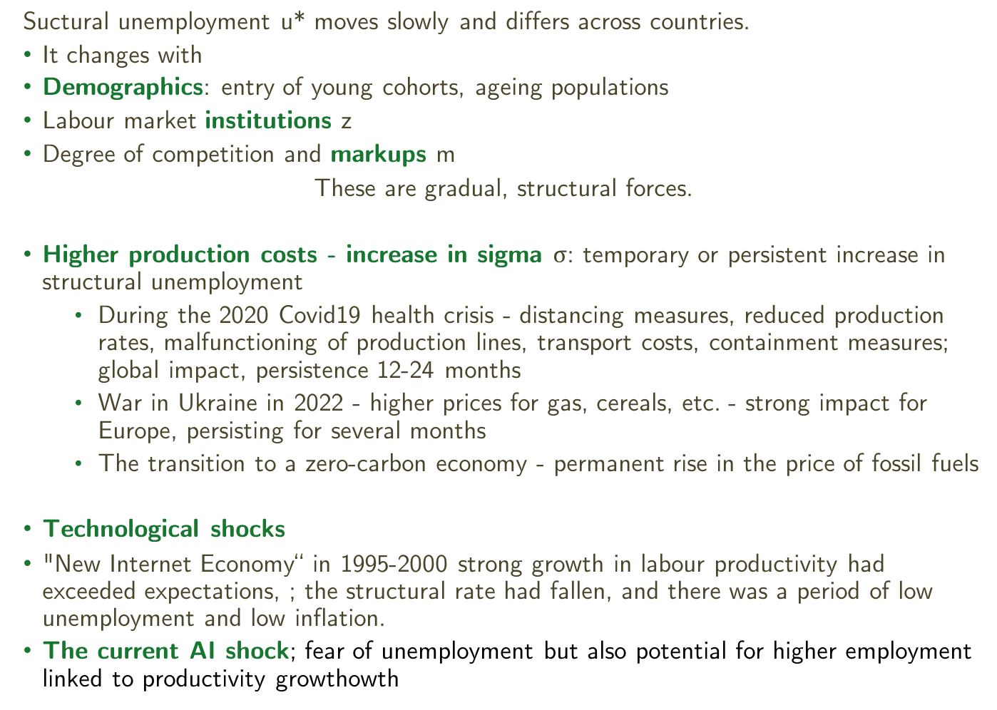
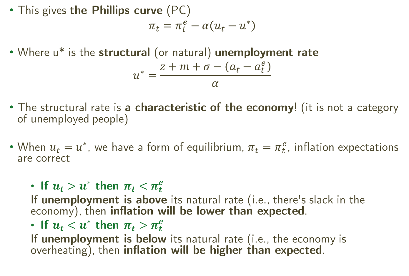
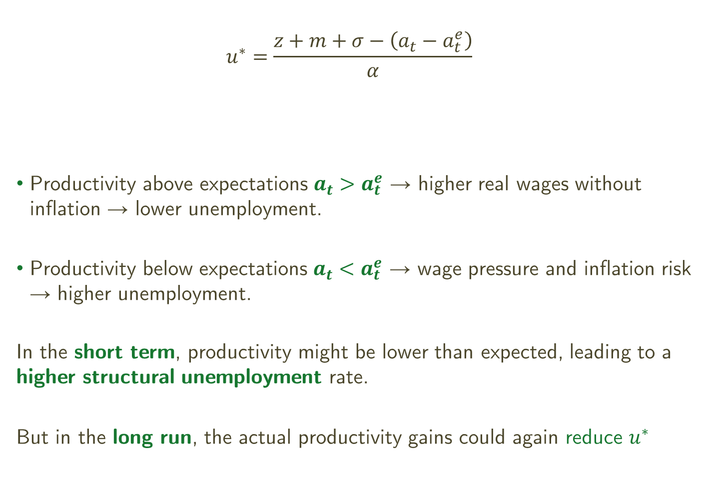
\(u^*\)Structural unemployment (NAIRU)The unemployment rate at which inflation is stable. \(u^* = \frac{m + z + \sigma - (a - a^e)}{\alpha}\).
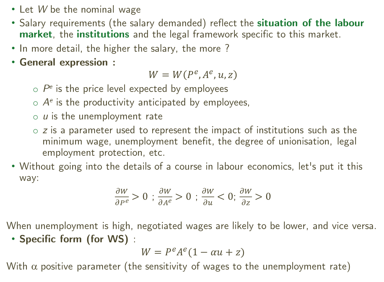
\(W\)Nominal wageWage in euros set by bargaining (WS curve): \(W = P^e A^e (1+z)(1 - \alpha u)\). Rises with expected prices, expected productivity and institutions; falls with unemployment.
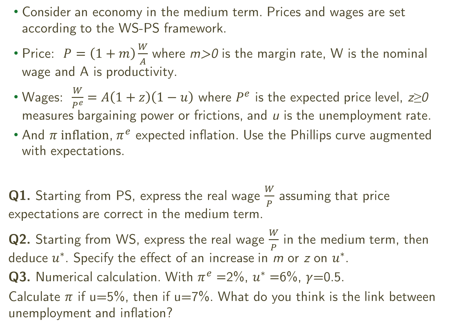
\(W/P\)Real wagePurchasing power of the wage. The PS curve pins it down: \(\displaystyle W/P = \dfrac{A}{(1+m)(1+\sigma)}\). Equilibrium \(u^*\) is where WS-real-wage = PS-real-wage.
\(P^e\)Expected price levelPrice level anticipated by wage-setters. If \(P^e = P\) (correct expectations) the economy sits at \(u^*\). Anchoring \(P^e\) is the central bank's core job.
\(A\)Labor productivityOutput per worker in the WS-PS model. Higher \(A\) raises the PS real wage. (In Solow, \(A\) is total factor productivity — same letter, related idea.)
\(A^e\)Expected productivityProductivity anticipated by workers when bargaining. Enters the WS curve. A positive surprise (\(a > a^e\)) temporarily lowers \(u^*\) — the late-1990s "Goldilocks" episode.
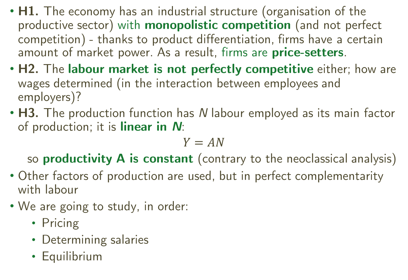
\(m\;(\text{markup})\)Firm markupProfit margin over marginal cost. Higher in more concentrated markets. In PS: \(\displaystyle P = (1+m)(1+\sigma)\,\dfrac{W}{A}\). Higher \(m\) → higher \(u^*\).
\(\sigma\)Supply-cost factorCaptures supply-side cost shocks and social charges in the PS curve \(P = (1+m)(1+\sigma)\,W/A\) (e.g. oil price, payroll taxes). Higher \(\sigma\) → higher \(u^*\).
\(z\)Labor market institutionsUnions, unemployment benefits, minimum wage — all push wages up at given \(u\). Higher \(z\) → higher \(u^*\).
\(\alpha\)Wage sensitivity to unemploymentSlope parameter of the WS curve. Higher \(\alpha\) → wages react more strongly to \(u\) → lower \(u^*\), steeper Phillips curve.
\(a,\,a^e\)Productivity growth (actual / expected)Growth rates of \(A\) and \(A^e\). The gap \((a - a^e)\) shifts \(u^*\): a positive surprise lowers structural unemployment until expectations catch up.
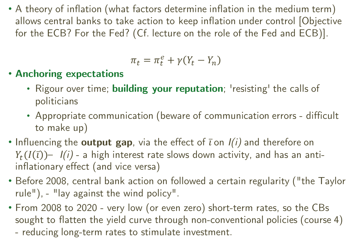
\(\gamma\)Phillips curve slopeOutput-gap form: \(\pi_t = \pi_t^e + \gamma\,(Y_t - Y^*)\), with \(\gamma = \alpha/(A\,L) > 0\). Links the output gap to inflation pressure.
\(L\)Labor forceTotal active population (employed \(N\) + unemployed). Used in \(u = (L-N)/L\) and potential output \(Y^* = A\,L(1-u^*)\).
\(r^*\)Natural (Wicksellian) interest rateReal rate at which \(Y = Y^*\) and inflation is stable. Target for central bank policy.
\(\psi\)Risk premium (project financing)Spread firms pay above the policy rate when borrowing. Lending rate \(= \bar{\imath} + \psi\).
SymbolNameDescription
\(e\)Nominal exchange ratePrice of foreign currency in domestic units. \(e \uparrow\) = domestic currency depreciates.
\(\varepsilon\)Real exchange rate\(\displaystyle \varepsilon = \dfrac{e\,P^f}{P}\). Relative price of foreign vs domestic goods. \(\varepsilon \uparrow\) = real depreciation.
\(\hat{e}_{t+1}\)Expected future exchange rateAnchor for the UIP relationship. Often treated as constant in short-term analysis.
\(i^f\)Foreign interest rateInterest on foreign risk-free assets. Key driver of capital flows in UIP.
\(X\)ExportsGoods/services sold abroad. Increasing in \(\varepsilon\) (real depreciation makes exports cheaper abroad).
\(IM\)ImportsGoods/services bought from abroad. Decreasing in \(\varepsilon\).
\(NX\)Net exports (trade balance)\(NX = X - \varepsilon \cdot IM\) in real terms. Medium-run Marshall-Lerner condition: \(|\varepsilon_X| + |\varepsilon_{IM}| > 1\).
\(\Delta A^{\text{dom}}\)Net financial inflowsForeigners' net acquisition of domestic assets. Counterbalances the current account.
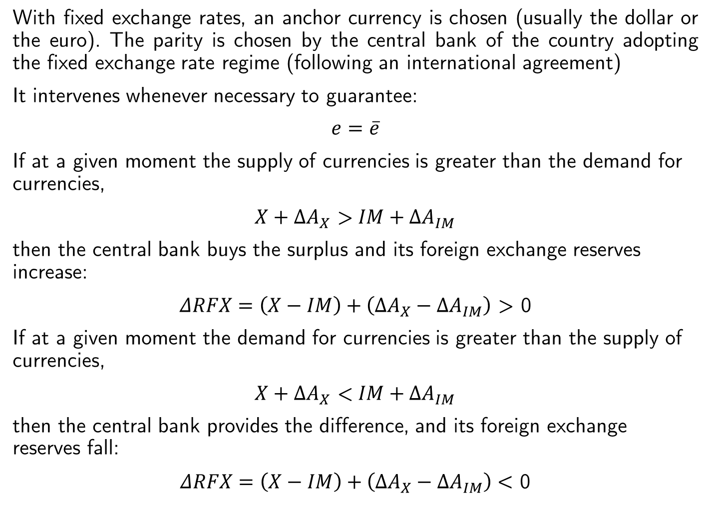
\(\text{RFX}\)Foreign exchange reservesStock of foreign currency held by CB. Changes under fixed exchange rate regimes to defend the peg.
SymbolNameDescription
\(K\)Capital stockTotal physical capital in the economy. Accumulates via investment, depreciates at rate \(\delta\).
\(N\)Labor (workforce)Number of workers. Grows at rate \(n\) (population growth).
\(A\)Total factor productivity (TFP)Exogenous technology parameter. Growth rate \(\bar{g}_A\) is the ONLY source of sustained per-capita growth in Solow.
\(k\)Capital per worker\(\displaystyle k = \dfrac{K}{N}\). Central variable in Solow model. Converges to \(k^*\) in steady state.
\(y\)Output per worker\(\displaystyle y = \dfrac{Y}{N} = f(k)\). Labor productivity.
\(s\)Savings rateFraction of output saved (= invested). Exogenous in Solow. Higher \(s\) → higher \(k^*\) but lower consumption in the short run.
\(\delta\)Depreciation rateFraction of capital stock that wears out per period. Combined with \(n\) to give "effective depreciation" of \(k\).
\(n\)Population growth rate\(\Delta N / N\). Dilutes capital per worker — must be offset by savings.
\(\alpha\)Capital shareExponent in Cobb-Douglas: \(Y = K^\alpha N^{1-\alpha}\). Empirically ~0.33.
\(k_{\text{gold}}\)Golden rule capital stockThe \(k^*\) that maximizes steady-state consumption. Condition: \(f'(k_{\text{gold}}) = n + \delta\).
\(E\)CO₂ emissionsTotal carbon emissions. Decomposed via Kaya identity.
\(W\)Energy useTotal energy consumption. In Kaya: \(E/W\) = carbon intensity of energy, \(W/Y\) = energy intensity of GDP.
\(\text{SCC}\)Social Cost of CarbonMarginal damage of 1 extra tonne of CO₂. The "right" carbon price per IAMs. Nordhaus: ~USD 59/tCO₂ starting, USD 125 by 2050.
💵 Money Market Equilibrium
Chapter 4 — How interest rates are determined
📘 Why hold money?
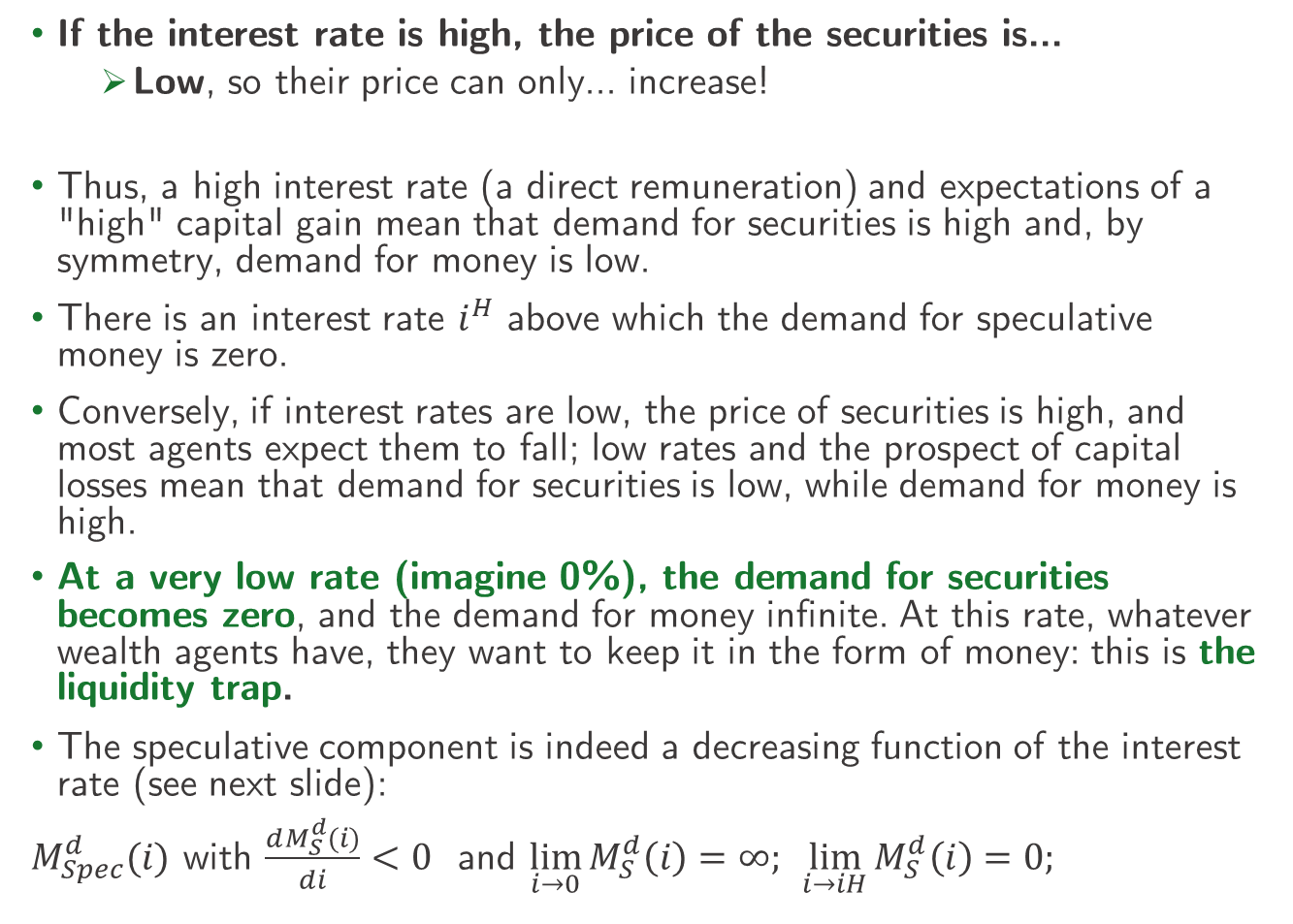
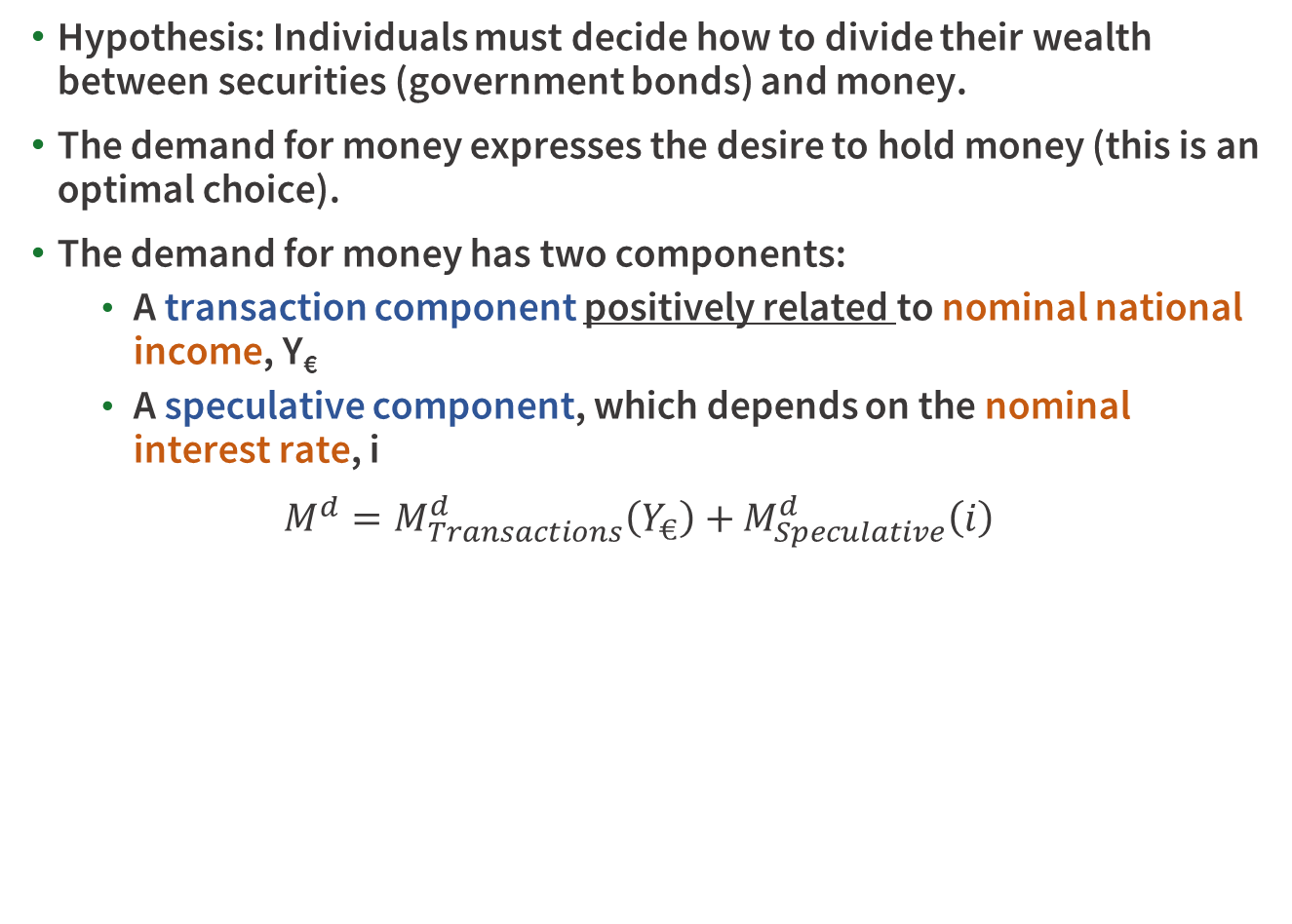
Money pays no interest, yet people hold it. Three motives: 1. Transaction — money is needed to buy goods (proportional to nominal income \(Y_{€}\)). 2. Precautionary — buffer against uncertainty. 3. Speculative (Keynes) — if \(i\) is high, people prefer bonds; if \(i\) is low, they hold cash expecting bonds to lose value.
🔢 Money demand function
\(M^d = M^d(Y_{€}, i)\) with \(\partial M^d/\partial Y > 0\) and \(\partial M^d/\partial i < 0\).
Linear form: \(M^d = kY_{€} - li\). Multiplicative: \(M^d = Y_{€}L(i)\) where \(L(i)\) is the "liquidity preference".
🧠 Bond prices and interest rates
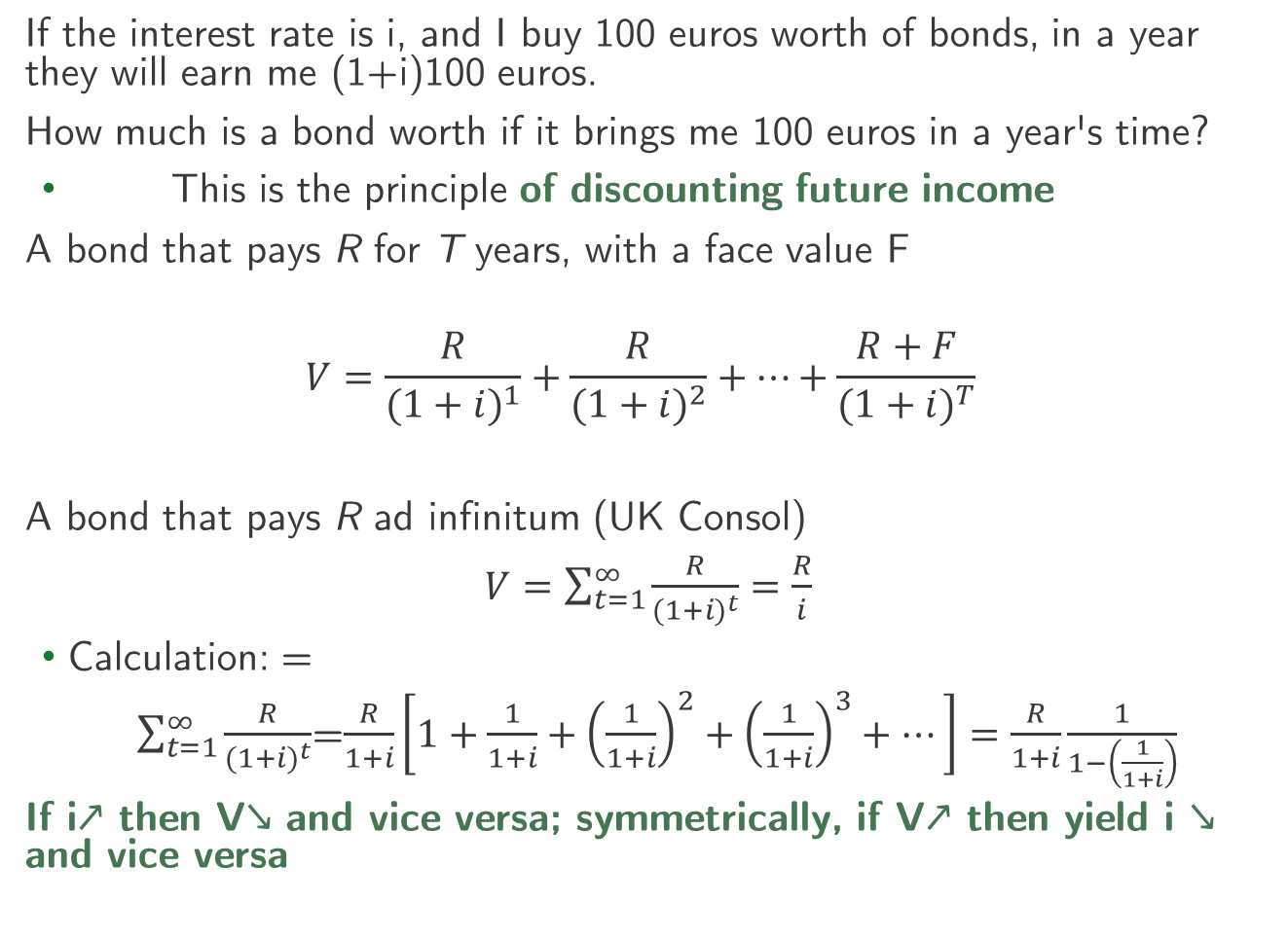
A 1-year bond paying €1000 at maturity has price \(P_B = 1000/(1+i)\). Key relationship: if \(i\uparrow\), then \(P_B\downarrow\). They move in opposite directions. A perpetual bond (UK Consol) paying \(R\) forever is worth \(P_B = R/i\).
📘 Money market equilibrium
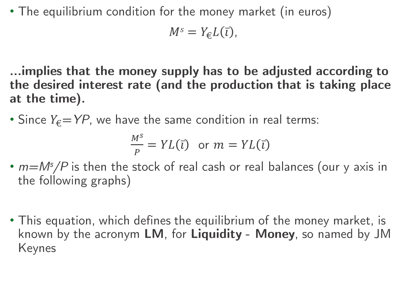
Central bank sets money supply \(M^s = \bar{M}\). Equilibrium: \(\bar{M} = Y_{€}L(i)\). If \(i\) is above equilibrium → excess supply of money → people buy bonds → \(P_B\uparrow\) → \(i\downarrow\) (adjustment to equilibrium).
⚠️ The liquidity trap
At i = 0 (zero lower bound), money demand becomes infinitely elastic (horizontal). People hold all extra money because bonds bring no return and could lose value if i rises. Conventional monetary policy becomes ineffective — fiscal policy becomes critical. Post-2008 era is the premium example.
🔢 The LM curve
At constant real balances \(\bar{m} = \bar{M}/P\), equilibrium gives a positive \((Y, i)\) relationship:
\(\bar{m} = YL(i)\) → slope \(di/dY = -L(i)/[YL'(i)] > 0\).
Higher \(Y\) → higher money demand → higher \(i\) for equilibrium.
🎯 Modern reversal
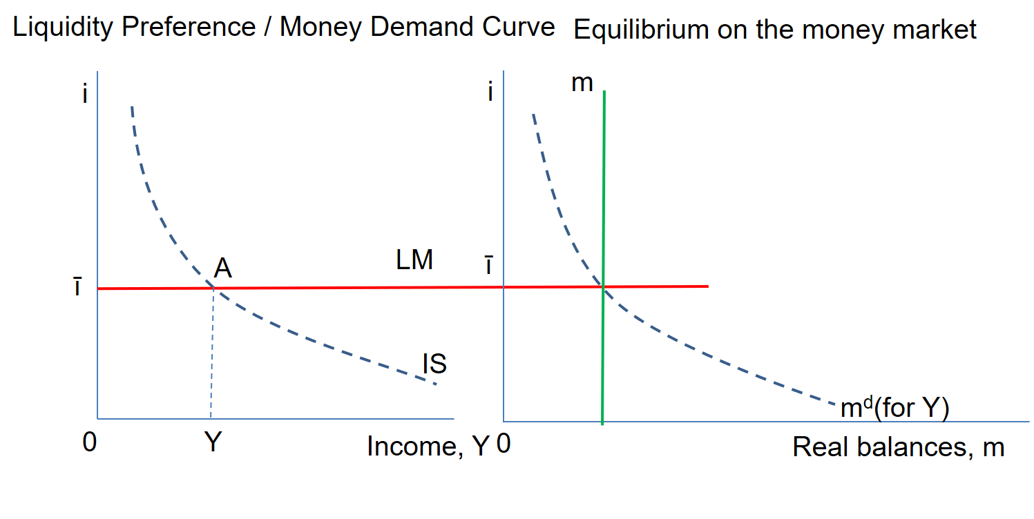
Since the 1990s, most central banks (Fed, ECB, BoE) no longer target \(\bar{M}\) directly. They choose the short-term interest rate \(\bar{\imath}\) and adjust \(M^s\) endogenously to hit it. The "pseudo-LM" becomes a horizontal line at \(\bar{\imath}\).
🏛️ Monetary Policy in Practice
Chapter 5 — How central banks really work
📘 Conventional tools (ECB)
Three main instruments: 1. Main refinancing operations (MRO) — short-term loans to banks, at the policy rate. 2. Marginal lending facility — banks' emergency overnight borrowing (ceiling). 3. Deposit facility — rate paid on bank reserves (floor).
The three rates form a corridor around the target policy rate.
📘 Unconventional tools (post-2008)
LTRO (Long-Term Refinancing Operations) — multi-year loans to banks. QE (Quantitative Easing) — CB buys bonds on the market, pushing up prices and pushing down long-term yields → flatten the yield curve. Forward guidance — communicating future policy intentions to shape expectations.
🧠 Why QE?
When \(i = 0\), conventional policy is stuck. QE works through a different channel: by buying long-term government bonds, the CB lowers long-term yields, stimulating investment and asset prices. The ECB balance sheet peaked at €8,800bn in Dec 2021 (vs. €1,200bn in 2007).
⚠️ Transmission lag
Monetary policy effects appear with a lag of ~18 months. This makes fine-tuning the economy extremely difficult. A CB raising rates today is fighting expected inflation, not current inflation.
🎯 Know the institutional setup
Fed: dual mandate (price stability + maximum employment). Run by the FOMC, meets 8 times/year. ECB: primary mandate = price stability (2% HICP target). Secondary: support general EU policies. Governing Council decides. BoE: MPC (Monetary Policy Committee), 2% CPI target.
📐 Inflation Theory & Phillips Curve
Chapter 6 — The inflation-unemployment trade-off
📘 WS-PS Labor Market Model
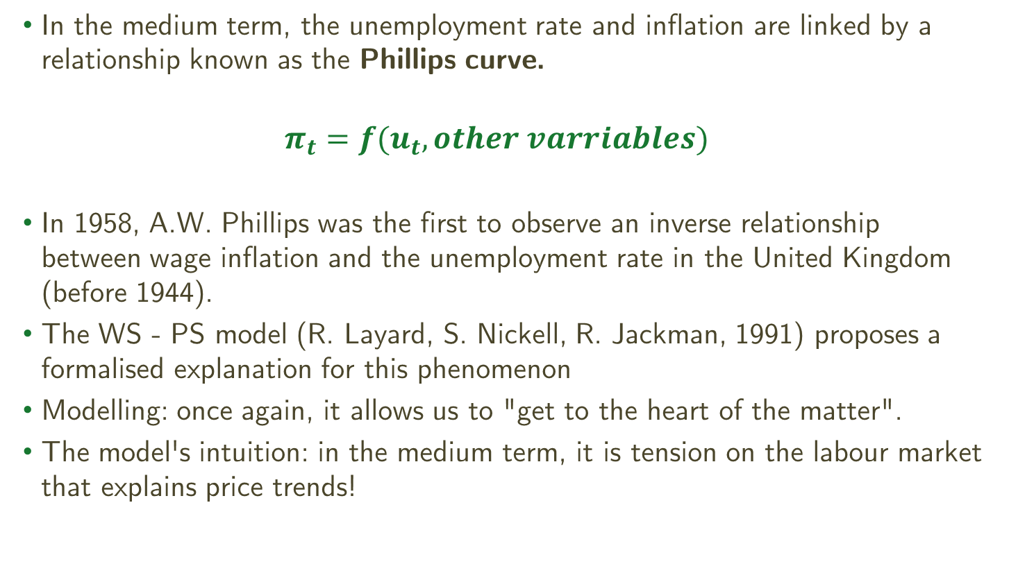
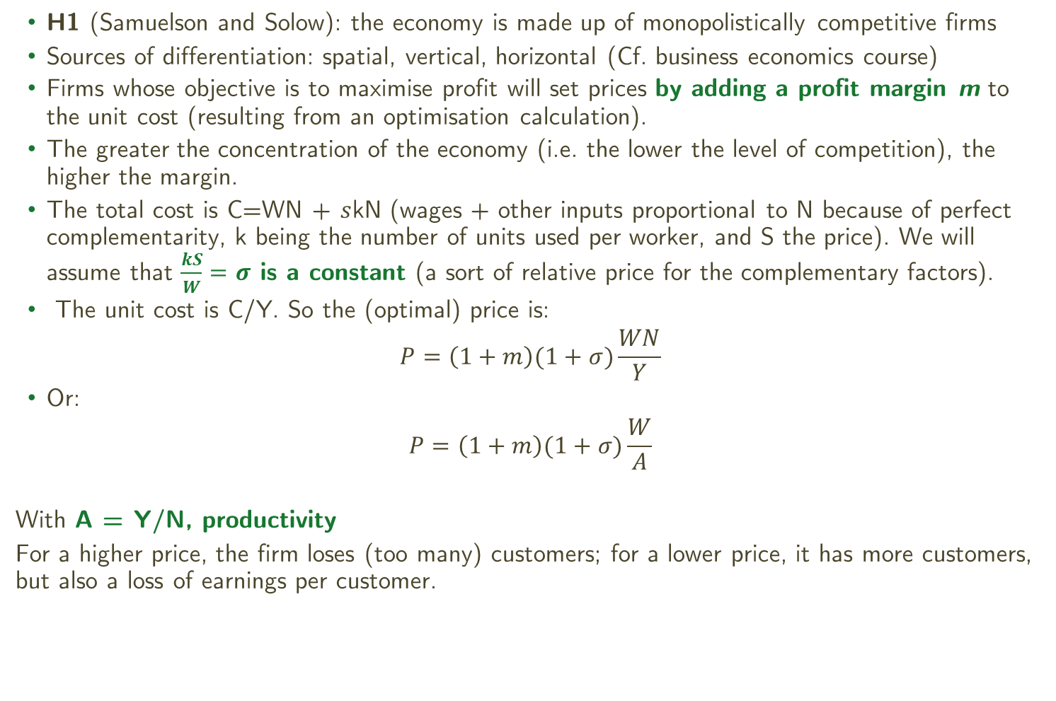
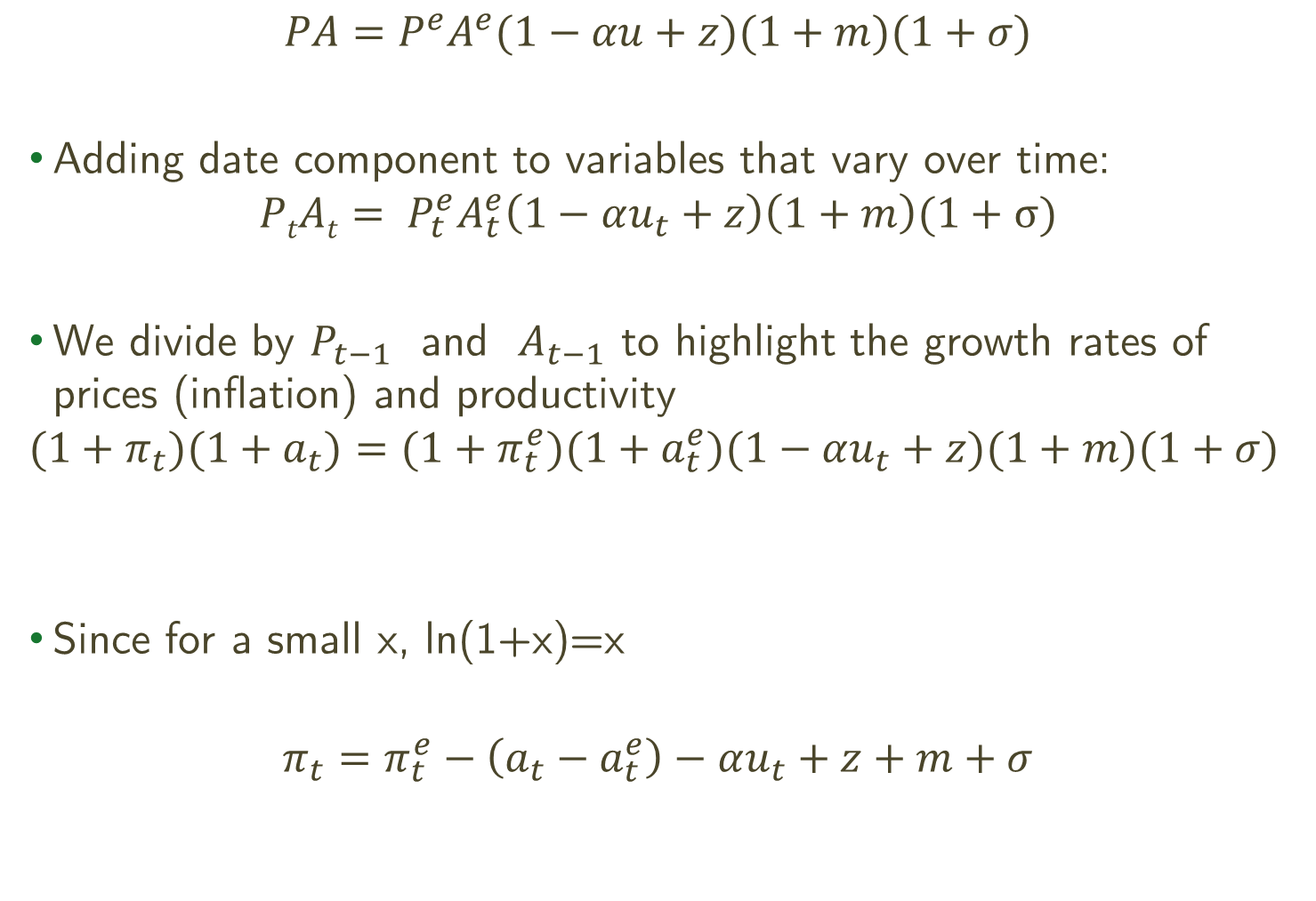
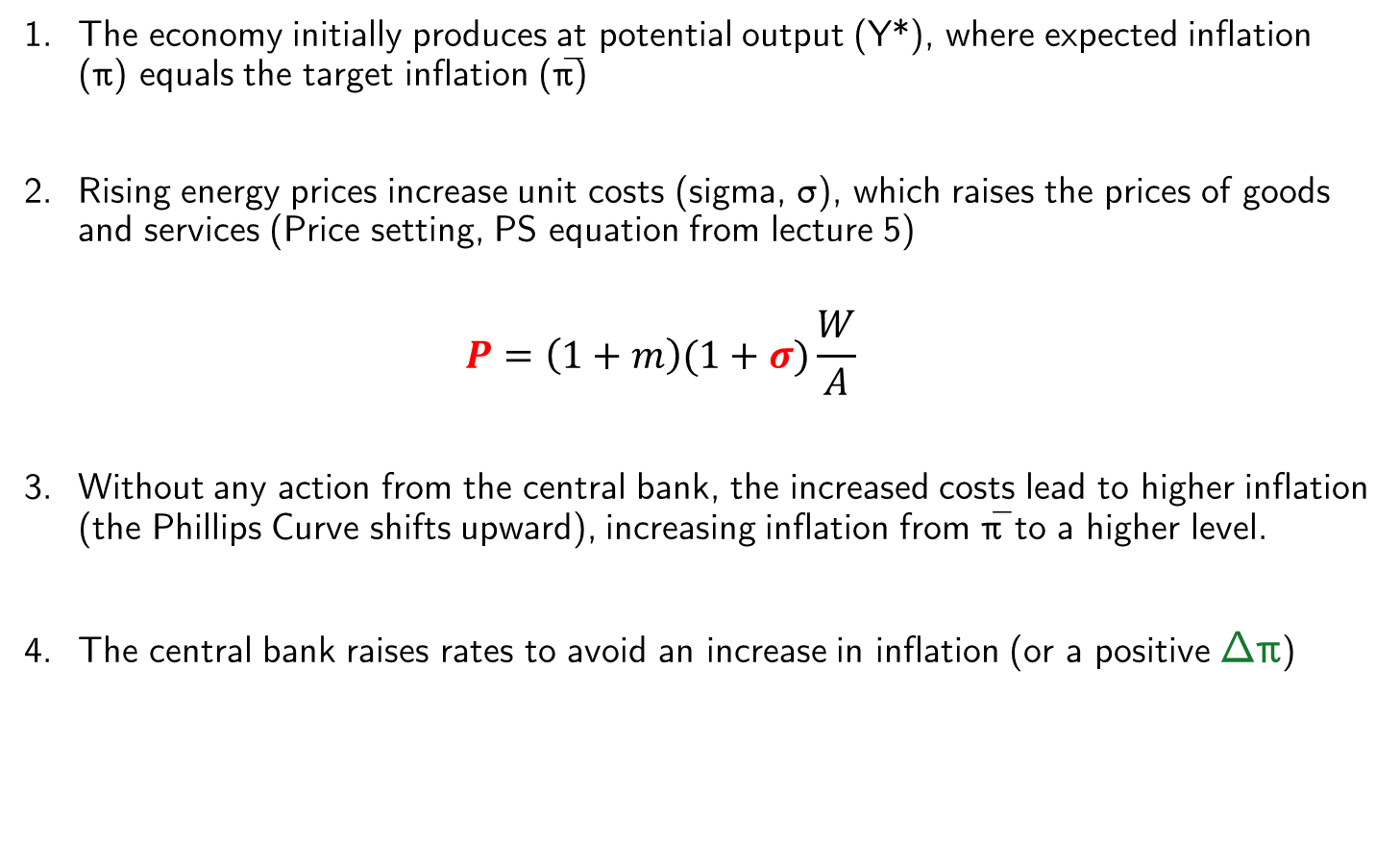
Price-Setting (PS): firms with market power set prices as a markup over unit costs: \(\displaystyle P = (1+m)(1+\sigma)\,\dfrac{W}{A}\), where \(m\) is the markup, \(A\) is productivity. Wage-Setting (WS): workers negotiate wages based on expected prices, productivity, unemployment, and institutions \(z\): \(W = A^e P^e(1+z)(1-\alpha u)\).
🔢 The Phillips Curve
Combining WS and PS yields the inflation equation:
\(\pi_t = \pi_t^e + \alpha(u^* - u_t)\)
Or with adaptive expectations (\(\pi^e = \pi_{t-1}\)):
\(\Delta\pi_t = \alpha(u^* - u_t)\)
🧠 What this means
When \(u < u^*\) (tight labor market), wages rise, then prices rise → inflation accelerates.
When \(u > u^*\), wages stagnate → inflation decelerates.
Only at \(u = u^*\) is inflation stable. This u* is the structural (natural) rate of unemployment, also called NAIRU (No-Accelerating Inflation Rate of Unemployment).
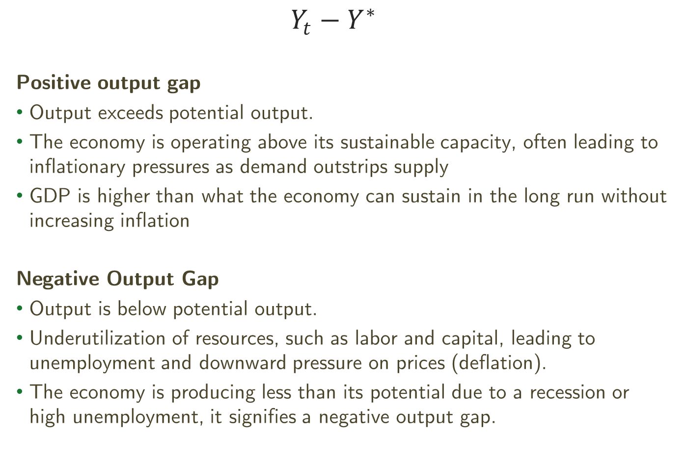
Demand-pull inflation: \(Y > Y^*\) (overheating) pushes inflation up along the curve. Cost-push inflation: supply shock (oil, \(z\), \(\sigma\)) shifts the whole curve up/left — inflation rises without output rising. Classic 1970s stagflation. The policy response is different for each!
🎯 Goldilocks & New Economy (1996-2000)
US had \(u \approx 3.9\%\) (very low) AND inflation ≈ 3.5% (low). Normally unexpected. Explanation: unexpected productivity surge (IT revolution) — \(a_t > a_t^e\) → temporary fall in \(u^*\). Robert Gordon (2012) measured 2.46% productivity growth 1996-2004, vs. 1.38% before.
⚖️ Medium-Term Equilibrium & Crises
Chapter 7 — The standard model applied to real crises
The real interest rate \(r^*\) at which \(Y = Y^*\) and inflation is stable (\(\Delta\pi = 0\)). When the CB sets \(r\) below \(r^*\), output overheats and inflation rises. When above, output cools and inflation falls. This is the "neutral" rate.
🧠 GFC 2007-2009 (demand crisis)
Subprime crash → banks hoard liquidity → credit dries up → \(\psi\) (risk premium) \(\uparrow\) sharply → IS shifts left → \(Y\) falls, unemployment rises. Fed cut rates to 0 (Dec 2008), launched QE. Still insufficient → fiscal stimulus needed. The zero lower bound exposed the limits of monetary policy.
🧠 Oil shocks 1973, 1979 (supply crisis)
Higher input costs → \(\sigma\uparrow\) → \(u^*\) shifts up → inflation equation shifts left: at any \(Y\), inflation is higher. Stagflation (high inflation + high unemployment). Policy dilemma: fighting inflation with rates deepens the recession.
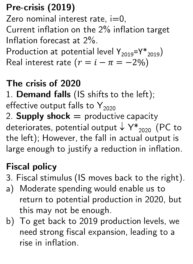
🧠 COVID-19 (2020, combined crisis)
Supply side: lockdowns, supply chain disruption, sanitary costs → shift left of inflation equation. Demand side: services demand collapses → IS shifts left. Unprecedented fiscal response (US: 26% of GDP stimulus) + monetary accommodation. Result: brief recession, then inflation surge in 2022.
⚠️ The 2022-23 inflation fight
US inflation peaked at ~9% (June 2022), Eurozone at ~10.6% (Oct 2022). Central banks raised rates aggressively: Fed from 0% to 5.25%, ECB from 0% to 4%. ECB was slower to react and later apologized. Inflation only came down after 18+ months — the transmission lag made it look like policy wasn't working.
🎯 Deflation spiral
At \(i = 0\), if inflation becomes negative (deflation), the real rate \(r = i - \pi^e\) actually rises! This chokes investment and deepens the recession, which deepens deflation. A self-reinforcing trap. This is why the ECB/Fed fear deflation more than moderate inflation.
🌍 The Open Economy
Chapters 8-10 — Exchange rates, UIP, J-curve, and policy
📘 Exchange rate conventions
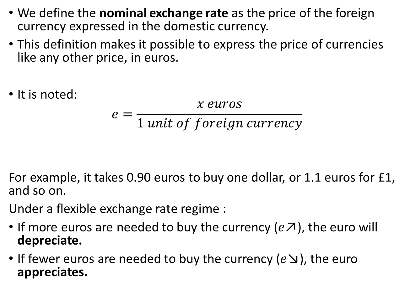
Nominal exchange rate \(e\): price of foreign currency in domestic currency (e.g., \(e = 1.20\) means 1.20 €/$).
If \(e \uparrow\): euro depreciates. If \(e \downarrow\): euro appreciates. Real exchange rate: \(\displaystyle \varepsilon = \frac{eP^f}{P}\) — accounts for price level differences.
🔢 UIP — Uncovered Interest Parity
Under perfect capital mobility, with expected future rate \(\hat{e}_{t+1}\):
\((1+i_t) = \dfrac{\hat{e}_{t+1}}{e_t}(1+i_t^f)\)
Solving: \(e_t = \hat{e}_{t+1} \times \frac{1 + i_t^f}{1 + i_t}\)
🧠 Intuition of UIP
If domestic \(i\) rises, investors buy domestic assets → domestic currency appreciates (\(e\downarrow\)). Higher \(i\) ⇒ stronger currency (in the short run, holding expectations constant). This is the key mechanism for understanding why ECB/Fed rate decisions move FX markets.
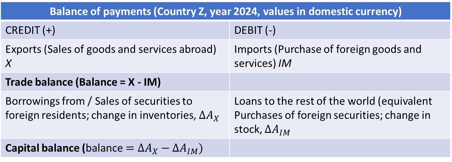
📘 Balance of payments
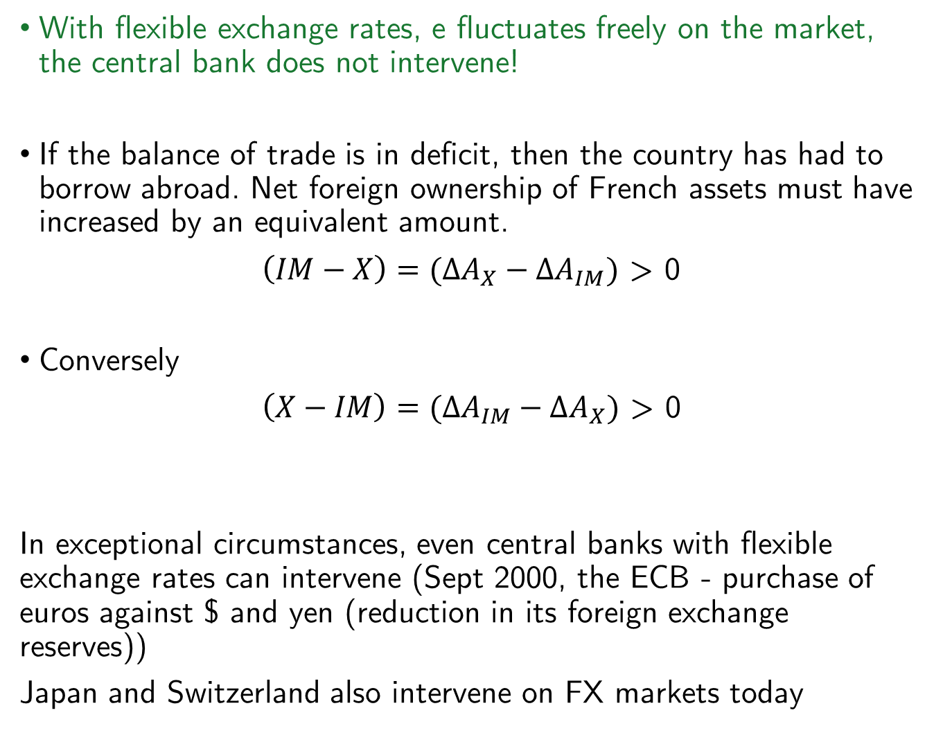
Always balanced by construction: Current account (trade + primary/secondary income) + Financial account = 0 (for flexible regimes).
A current account deficit must be financed by a financial account surplus (borrowing abroad).
📘 The J-curve
After a real depreciation (\(\varepsilon\uparrow\)), the trade balance initially worsens (price effect dominates — imports are immediately more expensive), then improves over time (volume effect — cheaper exports gain market share, dearer imports are substituted away).
🔢 Marshall-Lerner Condition
Real depreciation improves NX if and only if:
\(\left|\varepsilon_X\right| + \left|\varepsilon_{IM}\right| > 1\)
(sum of absolute values of export and import price elasticities exceeds 1). Empirically satisfied in most open economies in the medium run.
Tariffs were calculated proportional to bilateral trade deficits — economically flawed. Bilateral deficits reflect specialization and comparative advantage, not "cheating". Tariffs raise import prices, hurt consumers and firms using imported inputs, and typically trigger retaliation.
🧠 Fiscal policy under flexible rates
\(dG > 0\) → IS shifts right → \(Y\uparrow\) → money demand ↑. If the CB keeps \(i\) constant, \(e\) doesn't change. Fiscal policy works but with a caveat: higher \(Y\) → more imports → NX worsens. Some of the fiscal stimulus "leaks" abroad.
🧠 Monetary policy under flexible rates
\(di < 0\) (rate cut) → UIP: currency depreciates (\(e\uparrow\)) → NX improves → demand boosted by BOTH lower \(i\) (investment) AND weaker currency (exports). Monetary policy is very effective under flexible rates.
⚠️ Independent monetary policy is impossible
Under a fixed exchange rate regime, the CB must intervene (buy/sell FX) to maintain parity. If it tries to cut i, capital flees, currency comes under pressure, CB must sell FX reserves to defend the peg. The "impossible trinity": fixed rate + free capital mobility + independent monetary policy — pick 2.
🧠 Fiscal policy is very effective
\(dG > 0\) → demand rises → money demand rises → pressure on \(i\) upward → capital inflows → pressure on appreciation → CB buys FX to maintain peg, effectively increasing money supply endogenously. No crowding out, full multiplier effect.
📘 Trade-offs of each regime
Fixed pros: trade stability, anti-inflation anchor. Cons: no monetary autonomy, vulnerability to speculative attacks. Example: Bulgaria pegs Lev to Euro. Flexible pros: monetary autonomy, automatic absorber of shocks. Cons: volatility, speculative overshooting.
📈 UIP — Exchange rate vs. domestic interest rate
Formula: \(e_t = \hat{e}_{t+1} \times \frac{1 + i_t^f}{1 + i_t}\). Move the sliders to see how e depends on i.
↑ \(i\) ⇒ the domestic currency appreciates (\(e\) falls). This is the base of short-term FX analysis.
🌐 Mundell-Fleming — IS-LM-BP (3 panels)
Open-economy model. The left panel shows standard IS-LM; arrows show adjustments under the selected exchange-rate regime.
Choose a regime and a shock to see the effect on the IS-LM-BP panel.
🌱 Solow Growth Model
Chapter 11 — The long-run engine of growth
🔢 Production function
\(Y = AF(K, N)\) with constant returns to scale.
Per capita: \(y = f(k)\) where \(y = Y/N\), \(k = K/N\). A common form: \(y = k^{\alpha}\) (Cobb-Douglas with \(0 < \alpha < 1\)).
🔢 Capital accumulation
\(\Delta k_{t+1} = sf(k_t) - (\delta + n)k_t\)
where \(s\) = savings rate, \(\delta\) = depreciation rate, \(n\) = population growth.
Capital per capita rises when investment \(sf(k)\) exceeds replacement needs \((\delta+n)k\).
📘 Steady state (k*)
Equilibrium where \(\Delta k = 0\): \(sf(k^*) = (\delta + n)k^*\). This gives stable long-run capital per worker.
In the steady state, output per capita is constant — growth only comes from technical progress!
🔢 Golden rule (\(s_{\text{gold}}\))
The savings rate that maximizes steady-state consumption. Condition:
\(f'(k_{\text{gold}}) = n + \delta\)
Marginal product of capital = population growth + depreciation. Saving more raises \(k^*\), but also eats into consumption; the golden rule balances these.
🧠 Key Solow insights
1. Capital accumulation alone can't sustain growth — diminishing returns bring any economy to a steady state. 2. Only technical progress (\(A\uparrow\)) sustains long-run per capita growth. 3. Convergence: poor countries should grow faster than rich ones, all else equal (empirically messy).
🔢 Growth accounting (Solow residual)
\(\dfrac{\Delta Y}{Y} = \dfrac{\Delta A}{A} + \sigma_K\dfrac{\Delta K}{K} + \sigma_N\dfrac{\Delta N}{N}\)
The "Solow residual" \(\Delta A/A\) is total factor productivity — the unexplained part, attributed to technical progress.
🎯 With exogenous technical progress
If \(A\) grows at rate \(\bar{g}_A\), then in steady state per-capita output \(y\) grows at exactly \(\bar{g}_A\). Capital and output grow at the same rate as labor productivity. This is why economists focus on R&D, education, and innovation for long-run growth.
🌡️ Growth & Climate Change
Chapter 12 — Integrating economics with climate science
📘 Key facts
CO₂ concentration: 280 ppm in 1750 → 425 ppm in Feb 2024 (NASA). Unchecked, forecasts reach 700-900 ppm by 2100 → 3-5°C warming. IPCC target: limit warming to 1.5-2°C, requires halving emissions by 2030 vs. 2010.
🔢 I-PAT identity
Emissions decomposition: \(E = (E/Y) \times (Y/N) \times N\)
Impact = Technology × Affluence × Population. Kaya identity (more precise): \(E = (E/W) \times (W/Y) \times (Y/N) \times N\)
where E/W = carbon intensity of energy, W/Y = energy intensity of GDP.
🧠 Why emissions keep rising
\(E/Y\) (emissions per GDP) has been falling — but slowly. Meanwhile \(Y/N\) (GDP per capita) and \(N\) (population) rise fast. The net effect: total emissions still grow. Decoupling is possible (some countries have managed it), but globally insufficient.
📘 Integrated Assessment Models (IAM)
Nordhaus's DICE model (Nobel 2018) combines: (1) physical laws (CO₂ → temperature), (2) demographic projections, (3) economic growth equations, (4) damage functions linking temperature to GDP loss. Used by the UN to simulate policy scenarios.
🔢 Social Cost of Carbon (SCC)
The marginal damage of one additional ton of CO₂ — the "right" carbon price. Barrage & Nordhaus (2024) estimates: optimal SCC starts at USD 59/tCO₂ (close to EU ETS price), rising to USD 125/tCO₂ by 2050. Higher for stricter temperature targets.
⚠️ Poverty vs. climate trade-off?
Eradicating extreme poverty (SDG goal) would raise global emissions by only ~1% (Bruckner and al. 2022). The real tension is with middle-class consumption growth, not with lifting the bottom billion out of poverty.
👥 Key Economists & Their Theses
Click any card to open a structured mini-course
John Maynard Keynes1883 – 1946
💡 Central idea
In a recession, demand determines output, not supply. Markets do not self-correct quickly — unemployment can persist because aggregate demand (C+I+G) is too low. Government spending can close the gap. Published in The General Theory of Employment, Interest and Money (1936).
📅 Historical context
The Great Depression (1929-33): US output fell by 50%, unemployment hit 25%. Classical economics said markets would self-correct. They didn't. Keynes provided intellectual justification for fiscal intervention.
🔧 Model
Equilibrium: Y = Yd = C₀ + c(1−t)Y + I + G. If Y < YFE, firms under-produce and workers are idle. Increasing G injects demand; the multiplier \(1/(1-c(1-t))\) amplifies each euro of spending into more than one euro of GDP.
📊 Equilibrium below full employment
🎓 Course link
Foundation of Sessions 1-3: goods market, multiplier, fiscal policy, and the IS framework.
🎯 Exam essentials
In a demand crisis, demand determines output
Multiplier: \(dY/dG = 1/(1-c(1-t))\)
Assumes rigid prices (P=1), Y < YFE
⚠️ Common confusion
Keynes ≠ "spend unlimited amounts." He advocated counter-cyclical policy. The model only applies to demand crises — using it on supply shocks is a classic policy mistake.
Simon Kuznets1901 – 1985
💡 Central idea
Invented national income accounting and GDP — the single most important macroeconomic statistic. Nobel 1971.
📅 Context
During the Great Depression, US policymakers had no idea how much the economy produced. Commissioned in 1931 to build the first national accounts.
🔧 Three equivalent approaches
Production: Σ value added. Expenditure: \(Y = C + I + G + Xn\). Income: wages + profits + taxes − subsidies. All three ≡ GDP.
📊 GDP three approaches
🎯 Exam essentials
GDP = final goods only (no intermediate consumption)
Nominal growth ≈ Real growth + Inflation
Merger doesn't change GDP — only the internal/external split changes
⚠️ Confusion
Kuznets himself warned GDP is NOT a welfare measure. It misses household production, inequality, environment, leisure, digital "free" goods.
Paul Samuelson1915 – 2009
💡 Central idea
The Keynesian Cross (45° diagram) — the visual proof that demand determines output. Pioneer of the neoclassical synthesis. Nobel 1970.
🔧 The 45° diagram
45° line = Ys = Y (identity). Demand Yd has slope c(1−t) < 1. Equilibrium at the intersection. Increasing G shifts demand up → dY > dG (the multiplier).
📊 Fiscal multiplier on the Cross
🎯 Exam essentials
45° = identity Ys=Y. Not a supply curve
dY > dG because of the multiplier cascade
A. W. Phillips1914 – 1975
💡 Central idea
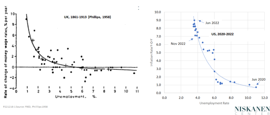
In 1958, documented the inverse relationship between unemployment and wage inflation in UK data. The Phillips Curve. Later augmented with expectations (Friedman/Phelps): the trade-off is temporary.
🔧 Expectations-augmented curve
πt = πte + α(u* − ut). Short run: trade-off exists. Long run: expectations adjust → economy returns to u*. Long-run Phillips curve is vertical at u* (NAIRU).
📊 Short-run vs long-run
🎯 Exam essentials
\(\Delta\pi = \alpha(u^* - u)\) with adaptive expectations
Short-run: trade-off. Long-run: vertical at u*
u* depends on labor institutions, markups, productivity surprises
⚠️ Confusion
Original Phillips (1958) = permanent trade-off. Modern (Friedman/Phelps) = temporary only. Never confuse the two in an exam.
Robert Solow1924 – 2023
💡 Central idea
Long-run per-capita growth cannot come from capital alone (diminishing returns). Only technical progress (↑A) sustains growth. Nobel 1987.
🔧 The Solow model
y = kα, dynamics: \(\Delta k = sf(k) - (\delta +n)k\). Steady state where \(s f(k^*) = (\delta + n) k^*\). Golden rule: f'(kgold) = n + δ. With tech progress at ḡA, steady-state y grows at exactly ḡA.
Only technical progress sustains per-capita growth
Solow residual = ΔA/A = unexplained part of growth
⚠️ Confusion
Higher savings raises k* (level effect) but NOT the growth rate (which stays ḡA). Don't confuse level and growth effects.
Olivier BlanchardAEA 2019
💡 Central idea
When i < g (nominal interest below growth), debt/GDP stabilizes automatically. The "global saving glut" made this hold pre-2022; high inflation reversed it.
Currently ECB ≈ 2%, French growth ≈ 0.9% → i > g (violated!)
Mundell & Fleming1960s — Nobel 1999
💡 Central idea
Extended IS-LM to open economies. The "impossible trinity": cannot have fixed FX + free capital + independent monetary policy. Pick two.
🔧 Policy implications
Flexible FX: monetary policy powerful (double channel: i + depreciation). Fixed FX: fiscal policy powerful (CB must accommodate). UIP: e = ê(1+if)/(1+i).
📊 The impossible trinity
🎯 Exam essentials
Flexible: monetary policy is king
Fixed: fiscal policy is king
Summers & Blanchard vs. Stiglitz2021 debate
💡 The inflation debate
Summers & Blanchard: Biden's stimulus (26% GDP) will overshoot potential → demand-pull inflation. Stiglitz: inflation is a "bogeyman." US inflation hit 8.9% (June 2022). Summers was right.
🔧 Logic
Aggregate demand >> potential supply → positive output gap → Phillips curve: \(\pi \uparrow \uparrow\). The Fed followed the "transitory" narrative and was slow to react. Political consequences: contributed to the 2024 Democratic defeat.
🎯 Exam essentials
Having a sound model enables correct predictions
Fiscal stimulus must be proportional to the output gap
Robert Lucas1937 – 2023
💡 Central idea
Rational expectations: agents use all info to forecast — only unexpected policy changes affect output. Growth rate differences dwarf all other welfare questions. Nobel 1995.
🎯 Exam
Income doubling: every 10 years (Korea 7%) vs 50 years (India 1.4%)
Systematic policy can't exploit the Phillips curve if expectations are rational
William Nordhausborn 1941
💡 Central idea
Pioneered the DICE Integrated Assessment Model linking economics to climate science. Social Cost of Carbon ≈ USD 59/tCO₂ optimal, rising to USD 125 by 2050. Nobel 2018.
🎯 Exam
IAMs combine physics + economics for climate policy
Kaya: \(E = (E/W)(W/Y)(Y/N)N\)
William Baumol1922 – 2017
💡 Central idea
Transaction cost model of money demand: fixed cost to convert bonds→money. Optimal balance trades conversion cost vs forgone interest. Result: Md decreasing in i — micro-foundation for the money demand curve (Ch.4).
David Ricardo1772 – 1823
💡 Central idea
Comparative advantage (1817): mutual gains from trade even if one country is worse at everything — specialize in what you do relatively best. Foundation of free trade theory. Context for Trump tariffs debate.
⚠️ Confusion
Comparative ≠ absolute advantage. Comparative advantage says nothing about the distribution of gains — free trade creates winners AND losers within each country.
Card, Angrist & ImbensNobel 2021
💡 Central idea
Quasi-natural experiments for causal inference. Card's minimum-wage studies overturned textbook predictions. Made economics a more rigorous empirical science. Key takeaway: correlation ≠ causation.
Robert Gordonborn 1940
💡 Central idea
Documented the IT productivity surge 1996-2004 (2.46% vs 1.38%). Unexpected productivity (a>ae) → u* fell temporarily → "Goldilocks economy." Broader thesis: post-1970 slowdown is structural.
Richard Baldwincontemporary
💡 Central idea
"Weaponization of interdependence" (2025): geopolitics now overrides efficiency in supply-chain decisions. Reshoring is structural. Higher production costs → potential ↑u* (σ↑).
Michael Spenceborn 1943
💡 Central idea
Nobel 2001 lecture: the art of modeling = choosing what to include. Too much → intractable. Too little → uninteresting. A meta-lesson on all macro models: know your assumptions.
Test your knowledge of the economists. Click the card to reveal, then rate your recall.
0
Remaining
0
Correct
0
Again
Question
Click to reveal answer
📉 Interactive Graphs
Explore economic models visually
Copy Method for Exam Charts
1. Name the axes Always write the horizontal variable, the vertical variable and the economic unit: Y, i/r, u, π, M/P, k, NX.
2. Set the initial balance Mark A, read the useful coordinates, then cite the equation which justifiess the intersection.
3. Identify the shock Demand, supply, fiscal policy, monetary policy, expectations, risk premium or productivity.
4. Move the right curve An endogenous variable causes movement along the curve; an exogenous variable shifts the entire curve.
5. Compare short and medium term Short term: Y may deviate from Y*. Medium term: inflation/expectations/rates return towards Y* or change Y*.
6. Conclude in one sentence Tell the final effect on Y, i/r, π, u, debt or NX. This is often where the easy points are won.
📐 Keynesian Cross — Goods Market Equilibrium
What happens? The 45° line is where Ys = Y (supply = income). The demand line Yd = C₀ + c(1−t)Y + I + G has slope c(1−t). Equilibrium is at the intersection. Increasing G shifts demand up → higher Y*. Why it matters: This diagram is the visual proof of the multiplier — notice that dY > dG because of the cascade effect through consumption.
📉 IS Curve — Interest Rate vs Output
What happens? The IS curve slopes downward: lower interest rate → more investment → more aggregate demand → higher equilibrium output. Increasing G shifts IS to the right. Why it matters: The IS curve is one half of the IS-LM model. Know how fiscal policy shifts it and how the slope depends on investment sensitivity (v) and the multiplier.
📊 Investment Function — I vs Interest Rate
What happens? Investment falls linearly as the interest rate rises: I = I₀ − vi. Higher v → steeper slope (investment is more sensitive to rate changes). Higher I₀ shifts the line right. Why it matters: This is the micro-foundation of why monetary policy works. The ECB/Fed lower rates → firms invest more → demand rises → GDP grows.
🔄 Multiplier Step-by-Step Animation
What happens? Each bar shows one "round" of the multiplier. The government spends dG, which becomes income, of which c is consumed, becoming new income, etc. The total converges to dG/(1−c). Why it matters: Exams ask you to trace the first 3-4 rounds. The geometric series logic is key.
📉 Public Debt Dynamics — Convergence vs. Snowball
What happens? If i < g (Blanchard's condition), debt/GDP converges to d̂ = σ(1+g)/(g−i). If i > g, debt snowballs — no finite steady state. Why it matters: Core Blanchard AEA 2019 insight. "Deficits matter, but i and g matter more."
📐 Phillips Curve — Inflation vs Unemployment
What happens? π = πᵉ + α(u* − u). When u < u*, inflation rises above expectations. Higher πᵉ shifts the whole curve up (expectations-augmented). Why it matters: Exams tests if you grasp that u* is the only stable unemployment rate (Δπ = 0). Below → accelerating inflation; above → disinflation.
💵 Money Market Equilibrium & Liquidity Trap
What happens? Money demand Md = kY − li slopes down. Supply M̄ is vertical. Intersection gives equilibrium i. When i hits 0, demand becomes horizontal (liquidity trap) — more money doesn't lower i further. Why it matters: Explains why QE was necessary post-2008: conventional policy was stuck at the zero bound.
💱 UIP — Exchange Rate vs Domestic Interest Rate
What happens? UIP: e = ê × (1+if)/(1+i). Higher domestic i → currency appreciates (e ↓). Higher foreign i or higher ê → domestic currency depreciates. Why it matters: Foundation of Mundell-Fleming model. Explains why monetary policy is powerful under flexible exchange rates.
↗ J-Curve — Trade Balance After Depreciation
What happens? At \(t_0\), the currency depreciates \((\varepsilon \uparrow)\). Initially, imports become more expensive immediately (price effect) — the trade balance worsens. Over time, volumes adjust: cheaper exports gain share, dearer imports are substituted — trade balance improves. Why it matters: Marshall-Lerner condition \(\left|\varepsilon_X\right| + \left|\varepsilon_{IM}\right| > 1\) determines if a depreciation ultimately helps. Usually yes in the medium run.
🌱 Solow Growth Model — Steady State
What happens? Steady state where investment sf(k) = depreciation needs (δ+n)k. Higher s raises k*. The "golden rule" savings rate maximizes steady-state consumption. Why it matters: Explains why growth slows as countries develop — diminishing returns to capital. Only technical progress (A↑) sustains long-run per-capita growth.
⚖️ Medium-Term: Natural Interest Rate r*
What happens? The IS curve gives Y as a function of r. The dashed vertical line is Y* (potential). If r̄ < r*, then Y > Y* → inflation accelerates. If r̄ = r* (natural/Wicksellian rate), inflation is stable. Why it matters: This is how CBs think about monetary policy — finding r*. Too loose (below r*) = overheating; too tight (above r*) = recession.
🗺️ Models Map — how it all fits together
The mental map for choosing the right model in review
Purpose of this page: avoid the classic mistake of knowing the formulas separately but not knowing when to use them. The course always moves from the demand for goods to rates, then to the labor market, inflation and crises.
🧭The logical thread of the course▼
1. National accounts Break down demand and measure activity.\(Y = C + I + G + X - IM\)
2. Goods market Understanding demand crises and multipliers.\(Y = A + c(1-t)Y\)
3. Rates and investment Linking the cost of financing to business decisions.\(I = I_0 + \mu Y - \nu i\)
4. Curve IS Transform the goods market into a decreasing relationship between Y and i.\(Y = f(i),\; f' < 0\)
5. Money, central banks and LM Understand how the rate is set or determined by liquidity.\(\dfrac{M}{P} = Y\,L(i)\)
6. WS-PS and structural unemployment Determine the level of activity compatible with labor-market institutions.\(u^* = (z + m + \sigma - (a - a^e))/\alpha\)
7. Phillips and IS-LM-PC Link output gap, inflation, natural rate and stabilization.\(\pi = \pi^e + \gamma(Y - Y^*)\)
8. Crises and policies Classify each shock: demand, supply or combination, then choose the instrument.\(r < r^* \;\Rightarrow\; Y > Y^* \;\Rightarrow\; \pi \uparrow\)
🔎Decision tree: which model to use?▼
Question about G, T, C, multiplier Use the Keynesian cross. Show initial shock, consumption rounds and final multiplier.
Question on investment or NPV Use the NPV rule and the I function. The rate increases the opportunity cost, so I decreases.
Question about Y-i relationship Use IS. An increase in G moves IS to the right; an increase in i causes a movement along IS.
Question on structural unemployment Use WS-PS. Institutions and margins determine u*, therefore Y*.
Question on persistent inflation Use Phillips. If Y > Y*, inflation accelerates; if Y = Y*, it is stable.
Question on crisis or policy mix Use IS-LM-PC. First classify the shock, then distinguish short term, inflation and return to Y*.
But : see what is exam ready, what is only covered in theory, and what still merits an exercise or chart. Statuses are calculated from file data, not from a vague impression.
Vital formulas, graphs to redo, priority exercises, pitfalls and backup
Target : produce an examination paper. The blocks below avoid the long course and only keep what earns points: model, calculation, graph, intuition, conclusion.
Loading exam mode...
🧮Vital formulas – to write without hesitation▼
📈Graphs — axis, shock, displacement, conclusion▼
🧪Priority Topics Teaching Notes▼
✅Copy checklist — score out of 10▼
🧑🏫Teacher proofreader — mark your copy before looking at the correction▼
0/10
Check the criteria actually present in your copy.
⚠️Pitfalls to review just before▼
Loading the save...
⏱️ Review Exam — 30 / 60 / 90 minutes
A filtered course that starts from your weaknesses and links directly to the right sessions, cards, quizzes and exercises
Principe : choose your available time. The file selects priority themes from the Weakness Dashboard, offers the most useful Teaching Notes exercises, then gives you direct buttons to review, test and memorize.
🎯Final sprint D-1 / D-0 — ultra-filtered▼
Loading the sprint final...
Loading the plan...
🧪Priority exercise queue▼
🔗 Cross-index — Sessions ↔ Themes
For each session of the course, the associated thematic sections (and vice versa)
For what ? There are two entries in this folder: by session (S1 → S6, like the Naef course) and by theme (GDP, IS, Phillips…). This index shows the correspondence to avoid revising the same thing twice and to avoid forgetting anything.
Note: Open Economy, Solow and Climate are not the subject of a dedicated Naef session in the 2026 program — review them directly via the thematic sections.
🧪 Exam Simulator — guided practice
Short topics, complete correction, and a score by theme
How to use it : topics are now constructed from Macro_Teaching_notes_2026-2.md. Choose a topic, answer mentally or on paper, reveal the correction, then grade yourself honestly. The dashboard will use these scores to tell you what to review first.
Loading the score...
Available topics
00:00
Theme
Subject
📝 Mock Exam — balanced subject 75 minutes
📊Historique de tes mock exams
A complete subject: calculation, model, graph, economic policy, trap
Objective : simulate a real copy. The topic is generated from the Teaching Notes exercises and graph drills; the correction returns to the simulator and the dashboard by skill.
75:00
Click on "Generate topic".
📈 Graph Drills — assessable graphs
Construct the graph: axes → initial equilibrium → shock → new equilibrium → conclusion
Exam rule: before clicking, draw the graph by hand. A graph earns points when you show what moves, why it moves, where the new equilibrium is, and what this implies for \(Y\), \(i/r\), \(\pi\), \(u\) or \(NX\). Geometry check: every equilibrium point must lie exactly on all curves/lines that define it.
No drill attempted.
🧮 Digital exercises — self-correction
10 typical exam calculations with automatic verification (tolerance ±1%)
How to use it : each exercise gives you parameters. Calculate on paper then enter your answer. The button checks immediately with a tolerance of 1%. The values change with each reload — no way to learn by heart.
🔄1 · Tax multiplier (endogenous tax)▼
Statement: An economy has a marginal propensity to consume and an endogenous tax rate . The government increases G by billion €. What is the variation in output ΔY (in € billion)?
Formula: \(dY/dG = 1/(1 - c(1-t))\)
📊2 · NPV of an investment project▼
Statement: A project requires an initial investment \(I_0 =\) M€. It generates a constant annual cash flow \(CF =\) M€ for 3 years. The discount rate is . Calculates the NPV (in €M, rounded to 0.01).
Formula: \(NPV = -I_0 + \Sigma CF/(1+i)^t\) for t = 1, 2, 3
📉3 · Dynamics of public debt (1 iteration)▼
Statement: Debt/GDP ratio initial \(d_{t-1} =\) (in %). Nominal interest rate , nominal growth rate . Primary balance \(sp =\) (as a % of GDP). Calculate d_t (in %, to the nearest 0.01).
Statement: Expectations inflation πe = . Observed inflation \(\pi =\). Structural unemployment \(u* =\). Sensitivity \(\alpha =\). What is the unemployment rate u (in %, to the nearest 0.01)?
Statement: Production function per capita \(y = k^\alpha\) with \(\alpha = 0.33\). Savings rate \(s =\). Depreciation \(\delta =\). Population growth \(n =\). Calculate the capital per capita k* in the steady state (to the nearest 0.01).
Statement: Money supply \(\bar{M}=\), price level \(P=1\). Income sensitivity , interest sensitivity . Real income \(Y=\). What interest rate i (in %) clears the money market?
Formula: \(\bar{M}/P = k\cdot Y - l\cdot i \Rightarrow i = (k\cdot Y - \bar{M}/P) / l \times 100 [in \%]\)
🌍10 · Real exchange rate \(\varepsilon\)▼
Statement: Nominal exchange rate (units of foreign per domestic). Domestic price level \(P=\). Foreign price level \(P^f=\). Compute the real exchange rate \(\varepsilon\) (±0.001).
Low score Return to the course exam sheet, redo the graph, then deal with two topics from the simulator.
Average score You know the idea but not yet the complete reasoning. Priority: write the steps and causalities.
Score strong Interview with flashcards and move on to exam traps. Don't hang on this topic for too long.
No data The theme has not yet been tested. Start a topic to avoid confusing confidence with real mastery.
🕯️ Exam watch — last consolidation
What you need to know to restore quickly, cleanly and without holes
Strategy : the day before, do not try to relearn the entire course. Your objective is to make the mechanisms automatic: recognize the model, write the equation, draw the graph, conclude economically.
🧮Formulas to take out without hesitation▼
GDP demand\(Y = C + I + G + X - IM\)
GDP income\(Y = \text{wages} + \text{profits} + \text{net taxes}\)
Budget recovery G increases autonomous demand, the demand line moves upwards, Y increases more than ΔG via the multiplier.
Increase in the key rate The real rate increases, investment falls, IS contracts, Y decreases; if Y < Y*, inflation decelerates.
Positive productivity shock A increases, PS becomes more favorable, u* decreases and Y* increases; this can reduce inflation for a given level of demand.
Negative supply shock Costs or margins increase, Y* falls and inflation rises: difficult trade-off for the central bank.
Credit crunch The risk premium increases the effective cost of credit, investment falls and IS shifts to the left even if the policy rate falls.
Sustainable debt It is not enough to look at the deficit: compare i and g, then integrate the primary balance.
Inflation persistante It comes from a lasting gap between Y and Y*, or from expectations which are revised upwards.
Covid Mixed shock: falling private demand, constrained supply, then exit with supply tensions and sustained demand.
⚠️Priority traps the day before▼
1
Movement vs displacement. A change in i moves the point to IS; a change in G moves IS.
2
Nominal vs. real. Investment decisions use the expected real rate, not just the nominal rate.
3
Deficit vs debt. The deficit is a flow; debt is an accumulated stock.
4
NAIRU vs observed unemployment. u* is structural; The current may deviate from it in the short term.
5
Supply shock treated as demand. Boosting Y without addressing supply can make inflation worse.
6
Forget expectations. In Phillips, πe moves the curve; it's not a detail.
7
Confondre r and r*. r* is the rate compatible with Y = Y*, not the rate chosen automatically.
8
Multiply without taxes. If t is endogenous, the multiplier becomes smaller.
9
Debt: forget g. GDP growth dilutes the debt-to-GDP ratio.
10
Graph without conclusion. The proofreader wants a final economic sentence, not just curves.
⏱️Last 60 minutes plan▼
0-15 min Review Models Map and minimal equations. Objective: choose the right model without hesitation.
15-30 min Redo three graphs: Keynesian cross, IS-LM-PC, Phillips. Trace them by hand.
30-45 min Do two simulator prompts in your weak themes. Read the correction, note the gaps.
45-60 min Read the priority pitfalls and model answers. Stop before saturating.
🃏 Flashcards — Spaced Repetition
🃏C'est le Main deck — 150 cartes transversales
Ce deck est global et mixte : il couvre TOUS les thèmes du cours (GDP, multipliers, IS-LM, Phillips, dette, croissance, climat…) en 150 cartes mélangées.
🔍 Différence avec les decks Naef S1-S6 : ces derniers sont séparés par session (12-18 cartes ciblées chacun, accessibles depuis ⏰ Due Today ou directement depuis chaque session Naef). Le Main deck sert à la révision croisée finale, quand tu veux mélanger les thèmes pour simuler l'exam.
Click the card to reveal the answer, then rate your recall
Normal mode: all due cards may fall.
0
Remaining
0
Correct
0
Again
Question
Click to reveal answer
✅ Quiz
Test your understanding — explanations after each answer
Normal mode: all questions are displayed.
Score: 0 / 0
⚠️ Top 10 Exam Traps
The mistakes students make most often
🎓 Typical Exercises — Teaching Notes
All course exercises classified by theme — with complete statements and solutions
📈
GDP & Indicators
⚙️
Keynesian model
📉
Debt & Stability
🏦
IS / Investment
📈 Theme 1 — GDP & Macroeconomic Indicators
🏭Ex. 1 — Calculation of GDP (steel mill + car manufacturer)Session 1 · GDP▼
📋 Statement (TN §1.3.1)
An economy is made up of two companies: a steel mill and an automobile manufacturer. The steel mill produces steel and sells it for a total of 100. It pays 80 in wages and makes a profit of 20. The car manufacturer sells cars for a total of 200. To produce them, it buys 100 of steel from the steel mill, pays 70 in wages and makes a profit of 30.
Questions: (1) Complete the value added tables. (2) Calculate GDP by value added. (3) Explain why total revenue ≠ GDP. (4) Calculate GDP by the income method. (5) What happens to GDP if the two companies merge?
✅ Solution
Steel mill value added: 100 − 0 = 100 (wages 80 + profits 20) Car manufacturer value added: 200 − 100 = 100 (wages 70 + profits 30) GDP by value added: 100 + 100 = 200 ≠ total revenue (100+200=300 = double counting !) GDP by income : wages (80+70) + profits (20+30) = 150 + 50 = 200 ✓ Merger: GDP = 200 (unchanged). Internal transactions disappear, but the final value added remains the same.
⚠️ Common exam pitfall
Adding revenues → double counting. GDP measures the net value created, not the total transaction volume. This is why we say "gross domestic product" and not "total revenue of the economy".
📊Ex. 2 — Nominal vs. real GDP (Calculation of growth rate)Session 1 · GDP▼
📋 Statement
A country produces in t-1: 100 units at 2€/u. In t: 110 units at 2.2€/u. Calculate: (1) Nominal GDP in t-1 and t. (2) The nominal growth rate. (3) The real growth rate (base t-1). (4) The implied inflation rate. Check the heuristic \(g_n \approx g_r + \pi\).
✅ Solution
GDP nominal t-1 : 100 × 2 = 200 | GDP nominal t : 110 × 2.2 = 242 \(g_n\): \((242-200)/200 =\) 21% Real GDP t (at price t-1): 110 × 2 = 220 \(g_r\): \((220-200)/200 =\) 10% π implicite : (2.2−2)/2 = 10%
Heuristic: 21% ≈ 10% + 10% = 20% ✓ (approximation for small values)
⚠️ Approximation or exact formula?
\(g_n = (1+g_r)(1+\pi) - 1\) exactly. The approximation \(g_n \approx g_r + \pi\) works well for low rates. For high values (e.g. hyperinflation), use the exact formula.
⚙️ Theme 2 — Keynesian Model & Multipliers
🛒Ex. 3 — Paradox of savingsSession 2 · Multipliers▼
📋 Statement (TN §2.7.5 Ex. 1)
Closed Keynesian economics. C = c(Y−T), exogenous investment I, exogenous taxes T. If households decide to save a larger fraction of their disposable income (c ↓), does total saving increase? Does the economy benefit? Show formally.
✅ Solution (TN Ex. 1)
Y* = 1/(1−c) × (C₀ − cT + I + G). If c ↓ → 1/(1−c) ↓ → Y* ↓.
Private savings: S = Y − T − C = (1−c)(Y−T). After decreasing c: Y* ↓ AND (1−c) ↑. The net effect: S may not increase, or even decrease if the fall in Y is sufficiently strong. Conclusion : What is individually rational (saving more) is collectively disructive. This is the savings paradox of Keynes.
Closed Keynesian economics. C = C₀ + c(Y−T), I and G exogenous. Study the effect of a simultaneous increase in public spending and taxes by the same amount: dG = dT > 0. What is the multiplier?
✅ Solution (TN Ex. 2)
Y = C₀ + c(Y−T) + I + G. By differentiating:
dY = c(dY − dT) + dG = c(dY − dG) + dG (puisque dT = dG)
dY(1−c) = dG(1−c) → dY/dG = 1 Interpretation: The initial net shock = dG − c×dT = dG(1−c) > 0. The drop in consumption due to taxes does not completely cancel out the increase in G because c < 1. Surprising result: growth without widening the deficit! (Valid in closed eco only.)
Two types of households. Rich: propensity to consume c < 1, receive share a of Y (with a > 0.5), pay taxes T. Poor: consume all their income (c = 1), receive share (1−a) of Y + transfer F from the government. Deficit = G + F − T. Questions: (1) Aggregate demand, (2) Balance Y*, (3) Effect of an increase in the share of the poor (da < 0), (4) Policy mix multiplier dT = dF.
✅ Solution (TN Ex. 3)
Y* = (F − cT + I + G) / [a(1−c)]
(3) if a ↘ → Y* ↗: poor households (c=1) have a higher propensity to consume, redistributing towards them stimulates demand.
(4) dY*/dT = (1−c)/[a(1−c)] = 1/a > 1 (because a < 1) The redistribution multiplier is greater than 1 — stronger than the standard balanced budget theorem. Source: The Economist "Trickle-up Economy" (Feb. 2020).
🛡️Ex. 6 — Unemployment benefits as an automatic stabilizerSession 2 · Stabilizers▼
📋 Statement (TN §2.7.5 Ex. 4)
Production Y = AN (A = constant productivity, N = employment). Active population L. Full employment: Y* = AL. Unemployment benefit B = δA per unemployed person (δ < 1 = replacement rate). Employees: CE = c(Y−T). Unemployed: CU = UB (consume everything). Show that the higher δ is, the more the fluctuations in Y due to investment shocks are damped.
✅ Solution (TN Ex. 4, eq. 2.38–2.39)
Y = c(Y−T) + δ(Y*−Y) + I + G (in substituant UB = δ(Y*−Y))
\(Y^* = \frac{1}{1-c+\delta}(I + G - cT + \delta Y^*_{\text{full}})\) dY/dI = 1/(1−c+δ)
As 1/(1−c+δ) < 1/(1−c), the investment multiplier is lower with δ > 0. The higher the replacement rate δ, the more stable the economy (unemployment benefits cushion shocks).
💸Ex. 7 — Covid-19 subsidies for American households (CARES Act)Session 2 · Fiscal policy▼
📋 Statement (TN §2.7.5 Ex. 6)
CARES Act (Trump, 2020) + American Rescue Act (Biden, 2021): checks of $600 then $1,400 to all Americans earning <$90,000/year. C = c(Y−T) + ηZ where Z = total amount of checks, η = propensity to consume the transfer. (a) Determine equilibrium Y*. (b) Compare the effect on consumption of a decrease in T, an increase in G, or an increase in Z.
✅ Solution (TN Ex. 6, eq. 2.46–2.48)
(a) Y* = 1/(1−c) × (I − cT + G + ηZ) (b) On consumption: effect of dG = effect of −dT (symmetric for equal deficit).
The effect of dZ on C is η/(1−c) (stronger if η > c). Conclusion : Checks are more effective on consumption than tax cuts if households consume more of their transfers (η > c). In practice, Americans saved their checks a lot (η < c) → stimulus less powerful than expected. Small open economies benefit less (import leakage).
👷Ex. 8 — Unemployment and income in the Keynesian modelSession 2 · Unemployment▼
📋 Statement (TN §2.7.5 Ex. 5)
Y = AN, A = constant productivity, N = employment. Active population L. U = L−N unemployed, each receives B euros. Unemployment insurance scheme in financial balance : T = B·U (employee taxes finance benefits exactly). Cemployees = c(Y−T), Cunemployed = BU (consume everything). No G. Questions: (1) Equilibrium employment N. (2) Effect of an increase in B on unemployment.
✅ Solution (TN Ex. 5, eq. 2.42–2.45)
(1) N* = [(1−c)BL + I] / [(1−c)(A+B)]
Condition for existence of unemployment: I < (1−c)LA (2) dN/dB > 0 (if unemployment > 0) Intuition : Increase B → the unemployed consume more (+1€ fully consumed) → demand ↑ → employment ↑. Paradox: more generous unemployment benefits reduce unemployment in this model! (Different from standard microeconomic logic.)
\(\sigma = 3\%\) of GDP (deficit), \(g_n = 5\%\) (nominal growth = real + inflation), \(i = 2\%\) (nominal interest rate). (a) Is the debt stability condition met? (b) To what value does the debt/GDP ratio converge? (c) What happens if growth increases by 1% point?
✅ Solution (TN Ex. 7, eq. 2.36)
(a) i = 2% < g = 5% → condition checked, the debt is stable. (b) d̂ = σ(1+g)/(g−i) = 0.03 × 1.05/0.03 = 1.05 = 105% of the GDP (c) g goes to 6%: d̂ = 0.03 × 1.06/0.04 = 79.5% of the GDP Lesson : An additional point of growth reduces the equilibrium debt by 25 points of GDP! Growth is the best remedy for public debt.
⚠️ Denominator sensitivity
The formula d̂ = σ(1+g)/(g−i) is very sensitive when g−i is close to 0. If g−i → 0, d̂ → ∞. This is why a slight reversal of the condition (i exceeds g) can cause a devastating debt crisis (Greece 2010, Türkiye, Argentina).
France 2026: debt D₀/Y = 115%, deficit σ = 6%, ECB rate i = 2%, nominal growth \(g_n \approx 1.5\%\) (0.9% real + approximately 0.6% inflation). (a) Is the stability condition met? (b) If the debt is not stable, what is the trajectory over 5 years? (c) What growth rate would be necessary to stabilize the debt at this deficit level?
✅ Solution
(a) i = 2% > g = 1.5% → condition no remplie → this diverges. (b) \(d_t = (1.02/1.015)\,d_{t-1} + 0.06 \approx 1.005\,d_{t-1} + 0.06\)
Trajectory: 115% → ~121% → ~127% → ~133% → ~139% → ~145% after 5 years. (c) So that d̂ = 115%: g − i = σ(1+g)/d̂ ≈ 0.06/1.15 ≈ 5.2% → g ≈ 7.2%! Almost impossible. France must reduce σ or refinance at lower rates.
🏦 Theme 4 — Investment & IS Curve
🏗️Ex. 11 — Investment projects and marginal rate of returnSession 3 · IS / NPV▼
📋 Statement (TN §3.1.1)
A company has 3 projects in its portfolio (cost + cash flows over several years):
Project
Cost
t=1
t=2
t=3
t=4
A
100
0
121
—
—
B
100
40
40
30
30
C
210
80
80
80
—
(a) Calculate î (marginal rate of return) for each project. (b) What projects should I carry out if i = 5%? If i = 15%? (c) Plot the investment function I(i) for i ∈ [0, 20%].
✅ Solution (TN §3.1.1, eq. 3.5)
Project A : 100 = 121/(1+î)² → (1+î)² = 1.21 → \(\hat{\imath}_A = 10\%\) Project B: \(\hat{\imath}_B = 16\%\) (numerical calculation) Project C: \(\hat{\imath}_C = 7\%\) (numerical calculation) (b) i = 5%: all projects (î > 5%) → I = 100+100+210 = 410
\(i = 15\%\): only B (\(\hat{\imath}_B = 16\% > 15\%\)) → I = 100 (c) Staircase function : I(i) = 410 if i<7% | 200 if 7%≤i<10% | 100 if 10%≤i<16% | 0 if i≥16%
🎯 Key message
Each project has a marginal rate of return î. A project is carried out if and only if the market rate i < î. Aggregating over all projects in an economy gives an investment function decreasing in i — the micro base of the IS curve.
Risk-free rate \(i_f = 1.5\%\). Probability of default \(p = 20\%\). Residual value in the event of a fault z = 0.40 (haircut 60%). (a) Calculate the risk premium ψ. (b) What happens if p doubles (40%)? (c) Perform for Greece 2012 (imposed haircut of 53.5%).
C = 50 + 0.7(1−0.3)Y, I = 100 − 200i + 0.1Y, G = 80. (a) Write the equilibrium condition Y = Yᵈ. (b) Solve for Y as a function of i. (c) Draw the IS curve. (d) What is the effect on Y if G increases to 110 (all i fixed)? (e) With LM: m = 0.5Y − 50i and m = 100, find the IS-LM equilibrium.
Macroeconomics studies how the economy works in its entirety. It is interested in aggregate indicators: total production, growth, inflation, unemployment. It analyzes the impact of monetary and budgetary policies, and the dynamics of economic structures over a long period.
💡 Why study it?
Firms : anticipate interest rates, exchange rates, labor market conditions. Investors : understand what bond and stock traders are thinking. Policy : design responses to crises. The macro has guided policies during every crisis since 1929.
Goods & services market: fiscal policy (G, T) Financial & monetary market: monetary policy (i) Labor market: determines inflation (link via the Phillips curve)
Interconnexion via IS-LM then Phillips.
📖 Methodology (TN §1.2)
Model : simplified representation of reality — "what to keep, what to leave out" (Spence, Nobel 2001). Endogenous variable: explained by the model (Y, i, u). Exogenous variable: external data (G, policies, demography). 3 types of relations : definitions, causalities, equilibrium conditions.
⚠️ Major crises to be aware of (TN §1.1)
1929–33 : Great Depression — unemployment 25% USA, industrial production −50%, bank runs. Origin of modern macro (Keynes). 1973 & 1979 : Oil shocks — stagflation (simultaneous inflation + unemployment). 2007–09 : Global Financial Crisis — subprime collapse, credit crunch. 2010–12 : Eurozone sovereign crisis — Greece, Ireland, Portugal, Spain. 2020 : COVID-19 recession — mixed supply + demand crisis. 2022–23 : Ukraine war, energy shock, inflation at 10%.
📈2. GDP — Gross Domestic Product▼
📖 Definition & origins
Measures the final production of resident units. Invented by Simon Kuznets (1931) at the request of the American government. "Understanding the Great Depression is the holy grail of macroeconomics" (Bernanke).
📖 GDP vs GNP
GDP: production generated within the territory. GNP: production by residents, wherever they are. Toyota factory in France → French GDP + Japanese GNP. GNP = GDP + NI (net foreign income). Ireland: GDP/GNP gap = −12% (multinationals).
3 equivalent approaches to GDP
$$Y = C + I + G + (X - IM) \quad|\quad Y = \sum \text{value added}_{\text{sectors}} \quad|\quad Y = \text{Wages} + \text{Profits} + \text{Taxes}$$
Nominal vs. real GDP (TN §1.3.1)
$$Y_N = Y \times P \;\Rightarrow\; g_n \approx g_r + \pi \quad \text{(heuristique fondamentale)}$$
🧮 Interactive GDP calculator — Added value
Company 1 (steel plant)
Company 2 (car manufacturer)
Total revenue (≠ GDP !)
—
CA₁ + CA₂
— + — = —
GDP (Σ Value Added)
—
(CA₁−m₁) + (CA₂−m₂)
— + — = —
GDP (Income)
—
w₁ + w₂ + π₁ + π₂
— + — + — + — = —
Adjust the settings to see how GDP is calculated.
⚠️ Limits of GDP (TN §1.3.1 & Economist 2016)
Does not measure: domestic production, informal economy, free goods (Wikipedia), quality of services (a candle vs. an LED — even "light" counted differently), inequalities, environment. But remains the reference crisis indicator to guide policies.
👷3. Unemployment — Definitions & Measurements▼
Key formulas (TN eq. 1.6–1.7)
$$L = U + E \quad|\quad u = U/L \quad|\quad \text{Employment rate} = E / \text{Working-age population}$$
📖 ILO Definition
Unemployed (ILO): unemployed + available within 2 weeks + actively looking for 4 weeks. THE discouraged leave the labor force (denominator L) → rate may fall during a crisis.
📖 Types of unemployment
Frictional : normal search time. Structural (u*) : natural rate/NAIRU — linked to institutional rigidities. Reference in the Phillips curve. Cyclical : u − u* = what Keynes seeks to reduce.
⚠️ Classic trap
The unemployment rate can lower during a crisis if discouraged workers leave the labor force (they are no longer looking → fall out of the denominator \(L\)). Always look at the employment rate (\(E/\text{population}\)) in addition. USA 1933: \(u = 25\%\). COVID 2020 peak USA: ~15%.
• \(w_i\) = weight of good \(i\) in the representative consumption basket (sum = 1). Re-estimated yearly via household surveys.
• \(\bar{w}_i\) = fixed base weight (reference period) — used to compare prices over time without basket composition polluting the measure (Laspeyres method).
• \(P_{i,t}\) = price of good \(i\) at period \(t\) (current month).
• \(P_{i,t-1}\) = price of good \(i\) at the previous period.
• \(i\) indexes the goods & services in the basket (~1,000 items in France, grouped into 12 categories: food, housing, transport, etc.).
📖 3 measures to distinguish
CPI — Consumer Price Index: representative household basket, the most widely used measure. HICP — Harmonized Index of Consumer Prices: harmonized across the euro zone, used by the ECB. Excludes owner-occupied housing (7.5% vs. 20% for the US CPI). GDP deflator — ratio \(Y_N / Y\) (nominal over real GDP): broader scope, covers all goods & services produced.
💡 Core inflation
Excluding energy and food (volatile). The ECB monitors core inflation for its decisions. In 2022: overall inflation 10.6% but core 5% → the ECB has raised rates. In 2026: inflation ≈ 2.5%, central bank rate ≈ 2%.
⚠️ Disinflation ≠ Deflation
Disinflation: π decreases but remains > 0 (prices rise again, more slowly). Deflation: π < 0 (prices fall). Deflation is dangerous: agents anticipate even lower prices → postpone purchases → demand fall → deflationary spiral (Japan 1990s).
📡5. Current Macroeconomic Conditions (2026)▼
🇺🇸 United States
Fed rate : 3.50–3.75%
Next FOMC meetings: April 28–29 & June 16–17, 2026
CPI inflation: ~4.2% (energy + Middle East war)
Uncertainty: Trump vs. Powell (Fed independence)
Eco policy: massive customs duties → record uncertainty
🇪🇺 Zone Euro
central bank rate : 2%
Next meetings: April 29–30 & June 10–11, 2026
Inflation zone euro : ~2.5% (mars 2026)
Lagarde : "We will not be paralysed by hesitation"
VIX: ~24 (high post-Trump trade uncertainty)
🎓 Question type "Starting question" (Naef)
"What do you think will be the ECB/Fed rate movement at the next meeting?" Complete argument: look at inflation (HICP vs 2%), growth prospects (g vs i for debt), the labor market (u vs u*), the geopolitical context (supply shocks = Trump tariffs). In April 2026: high uncertainty → probable status quo at the ECB.
CPI/IPC : representative consumer basket. PPI : producer prices, measured ex-factory, before taxes, transport and commercial margins. GDP deflator: implicit price of all domestic production: \(P = YN/Y\). Broader than the CPI, but less directly linked to the cost of living.
🔢 From statistics to variables
In models, statistics become abstract variables: \(Y_N\) for nominal GDP, \(Y\) for real GDP, \(P\) for general price level. The relationship \(Y_N = Y \times P\) allows the heuristic: nominal growth ≈ real growth + inflation.
💡 Why markets are looking at this data
Inflation, unemployment, GDP and policy rates move the prices of bonds, currencies and stocks. Persistent inflation pushes central banks to raise rates; an expected recession lowers yields and can increase demand for liquid assets.
⚠️ Signaux financiers of the PPTX
Gold : safe haven, but can be sold in a liquidity crisis to raise cash. VIX : measures financial uncertainty. Private debt / shadow banking : debt outside traditional banks, vulnerable if investors want to exit at the same time.
🃏Flashcards — Session 1▼
—
Remaining
0
Known
0
Again
S1 CARD—
Chargement…
Click to reveal the answer
⚠️Exam pitfalls — Session 1▼
1
Revenue ≠ GDP. Total revenue in an economy is not GDP — it double-counts intermediate inputs. GDP = Σ value added = Σ income.
2
Nominal GDP ≠ real GDP. An increase in nominal GDP can come from inflation alone. Always deflate to compare over time.
3
Low unemployment rate ≠ healthy labor market. The rate may fall if discouraged people leave the labor force. Also look at the employment rate.
4
Disinflation ≠ Deflation. Disinflation is π decreasing (but remaining > 0). Deflation is π < 0. These are two very different situations for monetary policy.
5
GDP = well-being? No. GDP measures market production, not well-being. But it is the best operational indicator to guide crisis policies.
📷Slides du cours — Session 1 (4 images)▼
Extraits du PPTX Alain Naef. Cliquer sur une vignette pour l'agrandir.
Bond prices and interest rates move in opposite directions. If i goes up, existing bonds are worth less in the secondary market. Traders adjust prices until yields equalize with the new rate.
🧮 Interactive calculator — Bond value
Value today \(V\)
—
—
Detailed calculation
—
Adjust the settings to calculate the bond value.
🎓 Course simplification (Naef)
We do not model the structure by run (yield curve) is vs risk premium. Monetary policy acts directly on short rates. Keynes hypothesis: financial wealth = money + public securities only.
💵2. The Demand for Mᵈ Currency▼
🛒
Transaction
Most liquid asset. If income Y ↑ → transactions ↑ → demand for money ↑.
\(\propto Y_\varepsilon\)
🛡️
Caution
Store of value. Zero return → arbitrage with securities that yield i.
Liquidity/yield trade-off
📈
Speculation
If i high → cheap bonds → prices can only go up → we buy securities rather than keeping M.
When i → 0: very high security prices → agents anticipate a drop → prefer to keep Mr. \(M^d_{\text{spec}} \to \infty\). Conventional monetary policy loses its effectiveness (2008–2021).
💡 Opportunity cost
Holding M costs i × M in uncollected interest. Not having M imposes a illiquidity cost \(C(M, Y_\varepsilon, s)\). Mᵈ optimal = point where the two costs balance.
⚖️3. Equilibrium on the Money Market — LM Curve▼
📖 Exogenous money supply (initial simplification)
The central bank controls supply: Mˢ = M̄ (vertical line on the graph). If it prints → M ↑ ; if it buys back via bonds → M ↓. In practice, banks also create money through deposits.
LM curve — in real terms (m = Mˢ/P, LM = Liquidity-Money)
$$m = Y\, L(\bar{\imath}) \quad\text{or}\quad m = k\, Y - l\, i$$
📊 Interactive chart — Money Market
Balance rate i*:—
Adjust the settings to see the adjustment mechanism.
Comparative statics
📈 Increase in income (dY > 0), constant Mˢ
Mᵈ increases → imbalance Agents sell bonds Bond prices ↓ → i ↑
💹 Hausse of Mˢ (dMˢ > 0), Y constant
Excess currency Agents buy bonds Bond prices ↑ → i ↓
📖 Modern monetary policy — Fixed CB ī
The large CBs (Fed, ECB) directly set the key rate ī. They adjust Mˢ to maintain this rate when Y fluctuates. On the IS-LM graph, the LM becomes a horizontal line at ī ("flat LM").
📐4. IS-LM Combined Model▼
💡 What changes vs session 3
Session 3 = IS alone, i exogenous. Here IS + LM = two equations, two unknowns Y and i. We can analyze the effect of policies on both variables simultaneously.
IS — goods market (reminder sessions 1–3)
$$Y = C_0 + c(Y - T) + I_0 + \mu Y - v\, i + G$$
LM — money market (session 4)
$$m = k\, Y - l\, i$$
IS solved — Y as a function of i
$$Y = \frac{1}{1 - c - \mu}\,(C_0 - cT + I_0 + G - v\, i)$$
3 key rates:
• Repo — 7 day loans to banks
• Deposit facility — yield on reserves
• Marginal lending facility — 24 hours (overdraft)
Unconventional instruments of the ECB
2012
OMT (Outright Monetary Transactions)
Conditional State Financing (ESM). Never used — ended the Eurozone crisis with his announcement alone. Draghi : "whatever it takes".
2022
TPI (Transmission Protection Instrument)
Supports the rise in post-2022 rates. Rapid assistance to States respecting stability rules to avoid fragmentation of spreads.
2014
European Banking Union
SSM (supervision of 110 large banks), SRM (rapid liquidation), deposit insurance (not yet in place).
🎓 Key point of the session
Liquidity trap = limit of conventional policy. 2008–2021: rates close to zero → QE, negative rates, OMT. Since 2022: return of inflation → increase in rates. Draghi's "whatever it takes" moment = the most important in the history of monetary policy according to Naef.
🧩PPTX supplements — mandates, balance sheets and monetary transmission▼
🇺🇸 Fed
The PPTX insists on the double mandate : price stability and maximum sustainable employment. The inflation target is around 2% on the PCE; since 2020, the Fed has accepted a logic ofaverage inflation targeting, therefore a temporary overshoot after a period below the target.
🇪🇺 central bank
Primary mandate: price stability, with the modern target of 2% symmetrical on the HICP since the strategic review of July 2021. The ECB can support EU economic policies only if this does not compromise price stability.
🏦 Bilan central bank
Assets: gold, foreign exchange reserves, purchased securities, refinancing loans to banks. Liabilities: bank notes and reserves. When the central bank buys assets or refinances banks, it creates reserves: the monetary base increases.
🏛️ Bank balance sheet
Assets: reserves, loans, securities. Liabilities: deposits, refinancing, equity. Banks transform liquid deposits into longer credits: this is useful for the economy, but it creates liquidity risk and justifiess reserves, capital and supervision.
Conventional instruments The Fed controls the Federal Funds market; the ECB uses the main refinancing rate, the deposit facility and the marginal lending facility. Before 2008, open market operations on short securities played a central role; after 2008, abundant reserves and the rate paid on reserves become decisive.
Unconventional instruments At the zero bound: forward guidance, LTRO/TLTRO, asset purchases and QE, sometimes negative rates. The objective is not only to lower the short rate: we must influence the entire rate curve, especially the long rates which weigh on investment, real estate and public debt.
🎓 Rate curve
Normal : long rates exceed short rates, often because the market demands a maturity premium or anticipates future increases. Flat : little change expected. Reversed : short rates exceed long rates, a classic signal of expectation of a slowdown and future rate cuts.
💡 Zone euro
The PPTX links OMT, PEPP, TPI and banking union to the same problem: preventing an increase in sovereign spreads from disrupting monetary transmission between countries. The mechanism can be announced without being used: if the promise is credible, it already reduces the risk premium \(x\).
🃏Flashcards — Session 4▼
—
Remaining
0
Known
0
Again
S4 CARD—
Chargement…
Click to reveal the answer
⚠️Exam pitfalls — Session 4▼
1
Bond price ≠ yield. When i goes up, the value V goes down. Very common confusion during the exam.
2
Mᵈ is decreasing in i — this is the opportunity cost. Not to be confused with the IS curve.
3
Liquidity trap ≠ absence of money. The currency exists, but the agents hoard it. The central bank can no longer lower i below zero (conventional policy).
4
Increase in income → increase in i if Mˢ constant. Do not say "Y↑ → i↓" without specifying that the central bank adjusts the offer.
5
Modern LM = horizontal line at ī. The central bank sets the rate and adjusts Mˢ. In realistic models, LM is no longer increasing.
📷Slides du cours — Session 4 (9 images)▼
Extraits du PPTX Alain Naef. Cliquer sur une vignette pour l'agrandir.
A demand crisis means \(Y \lt Y^{*}\): prices are fixed, unemployment rises and capital is underused. Demand determines output: \(Y=Y^{d}\).
Formulas
\[
\begin{aligned}
Y^{d} &= C + I + G + (X - IM)\\
C &= C_0 + c(Y - T)\\
Y &= \frac{C_0 + I + G + (X - IM) - cT}{1-c}\\
Y &= \frac{C_0 + I + G + (X - IM)}{1-c(1-t)}
\end{aligned}
\]
Chart
Know how to redo the Keynesian cross: \(45^\circ\) line, aggregate-demand slope \(c(1-t)\), an increase in \(G\) shifts demand upward in parallel, and \(\Delta Y \gt \Delta G\).
Question type
Calculate a multiplier, the effect of \(\Delta G\) on \(Y\), and the effect on the deficit. Always say if taxes are exogenous \(T\) or endogenous \(tY\).
Resolution method 1. Write \(Y=Y^{d}\). 2. Replace \(C\). 3. Bring the \(Y\)'s together on the left. 4. Factorize. 5. Identify the multiplier. 6. Conclude with intuition.
Fatal mistake Use \(\frac{1}{1-c}\) when the statement gives an endogenous tax rate \(t\), or forget that automatic stabilizers reduce the multiplier.
⚡
1. Nature of crises
📦
2. Demand
✖
3. Multiplier
🏛️
4. Fiscal
🛡️
5. Rules
⚡1. The nature of crises and the Keynesian reflex▼
📖 Definition
A macroeconomic crisis is a sharp drop in activity, measured by real GDP. A recession corresponds to two consecutive quarters of decline in GDP; a depression is a deeper and more persistent fall. The Keynesian response mobilizes fiscal policy and monetary policy.
💡 Diagnosis before remedy
Most of the historical crises studied are demand crises : Great Depression, GFC 2007-09, Eurozone sovereign crisis 2010-12. But supply crises exist: oil shocks, war in Ukraine, energy or logistical tensions. Covid combines the two.
Demand crisis C, I or X fall. Consequences: unemployment, bankruptcies, underutilization of capital, low inflation or deflation. Remedy: support demand.
Supply crisis Disrupted production costs or supply chains. Lower potential output, higher inflation. Demand stimulus alone is often unsuitable.
Mixed crisis Supply and demand move together. Covid 2020: confinement, absent workers, falling consumption and investment.
🎓 Cases and slide news
Hormuz/Iran illustrates a risk of a supply crisis via oil and transport. Eurozone 2008-10 and Covid 2020 show GDP losses. The central pitfall: using demand crisis measures in the face of a pure supply shock can worsen inflation.
📦2. Aggregate demand, assumptions and equilibrium▼
Complete aggregate demand
$$Y^d = C + I + G + (X - IM)$$
📖 The components
\(C\) : household consumption. \(I\) : business investment, residential real estate, inventory changes. \(G\) : public purchases of goods, services and capital, excluding transfers. \(X - IM\) : net exports. In session 2, we close the economy: \(X = IM = 0\).
🧮 Real exchange rate
The course already introduces open notation: \(\displaystyle \varepsilon = \frac{eP^*}{P}\). \(\varepsilon\) represents the quantity of domestic goods given to obtain one unit of foreign good. Nominal net exports are written \(PX - eP^*IM = P(X - \varepsilon IM)\).
Assumptions of the demand crisis model
H1. The economy is below full employment: \(Y < Y^*\).
H2. Rigid downward wages and constant prices: \(P = 1\).
H3. Horizontal supply: firms can produce more at the current price.
H4. Sales become income: \(Y^{s} = Y\), production-income identity.
H5. The interest rate is constant; investment is exogenous in this session.
In equilibrium, firms produce what agents want to buy: \(Y^{s} = Y^{d}\). As \(Y^{s} = Y\), we obtain \(Y = Y^{d}\). Demand therefore determines production, unlike a neoclassical reading where supply would be primary.
📊3. Interactive chart — Keynesian cross▼
Balance \(Y = Y^d\) with endogenous taxes
Adjust the parameters to visualize the balance shift.
✖4. Multipliers, deficit and balanced budget▼
Exogenous taxes T
$$Y = \frac{1}{1-c}\,(C_0 + I + G - cT)$$
Government spending multiplier
$$\frac{dY}{dG} = \frac{1}{1-c}$$
Tax multiplier
$$\frac{dY}{dT} = \frac{-c}{1-c}$$
Balanced budget multiplier (Haavelmo)
$$\left.\frac{dY}{dG}\right|_{dG=dT} = 1$$
Endogenous taxes t
$$Y = \frac{1}{1 - c(1-t)}\,(C_0 + I + G)$$
Multiplier with automatic stabilizers
$$\frac{dY}{dG} = \frac{1}{1 - c(1-t)}$$
Tax-rate multiplier (proportional)
$$\frac{dY}{dt} = \frac{-cY}{1 - c(1-t)}$$
Quick calculator
Multiplier
—
\(\Delta Y\) expected
—
📖 Deficit with exogenous taxes
\(Def = G - T\). An increase in \(G\) increases the deficit by 1:1; an increase in \(T\) reduces the deficit by 1 to 1. Example from the course: if \(c=0.8\), cutting \(G\) by 100 reduces \(Y\) by 500, lowering \(T\) by 100 increases \(Y\) by 400, net effect \(-100\).
🧮 Deficit with endogenous taxes
\(Def = G - tY\). An increase in \(G\) still increases the deficit, but less than 1:1 because \(Y\) increases and tax revenues increase. Key formula: \(dDef/dG = (1-c)(1-t)/[1-c(1-t)] > 0\).
🎓 Balanced budget theorem (Haavelmo)
Statement. In a closed Keynesian economy with exogenous taxes, if the State raises \(G\) and finances it exactly by raising \(T\) (\(dG = dT > 0\)), output rises by exactly the same amount: \(\boxed{dY = dG}\). The balanced-budget multiplier is 1 — activity expands without widening the deficit.
Proof. Start from the goods-market equilibrium with \(C = C_0 + c(Y-T)\), \(I\) and \(G\) exogenous:
$$Y = C_0 + c(Y - T) + I + G$$
Take the total differential (with \(C_0\), \(I\) constant):
$$dY = c\,(dY - dT) + dG$$
Apply the balanced-budget hypothesis \(dT = dG\):
$$\begin{aligned} dY &= c\,(dY - dG) + dG \\ dY - c\,dY &= -c\,dG + dG \\ (1-c)\,dY &= (1-c)\,dG \\[2pt] dY &= dG \;\;\Rightarrow\;\; \frac{dY}{dG}\bigg|_{dG=dT} = 1 \end{aligned}$$
Decomposition (why it works). The net first-round demand shock is the direct rise in G minus the fall in consumption caused by the tax hike:
Households cut consumption by only \(c\) of the tax rise (they finance the rest by reducing saving). This net shock is then propagated by the usual Keynesian multiplier \(\frac{1}{1-c}\):
$$\Delta Y \;=\; (1-c)\,dG \;\times\; \frac{1}{1-c} \;=\; dG$$
The \((1-c)\) at round 0 and the \(\tfrac{1}{1-c}\) of propagation cancel exactly — the multiplier collapses to 1, independently of \(c\).
⚠ Exam traps. (1) Result valid only in closed economy with exogenous T — opens with imports/endogenous taxes, the multiplier drops below 1. (2) The deficit \(G-T\) is unchanged, but the debt ratio \(d = D/Y\) falls because Y rises while D is unchanged. (3) The "neutral budget" intuition is wrong: even a tax-financed G expansion stimulates Y as long as \(c < 1\).
🛡️5. Fiscal policy in practice, stabilizers and limits▼
💡 How to stimulate demand?
Two fiscal levers, with very different transmission and very different multipliers.
① Public spending channel (\(dG > 0\)). \(G\) enters \(Y\) directly: 1 € of \(G\) = 1 € of demand at round 0, then propagated. Round-0 impact is full. Multiplier:
$$\frac{dY}{dG} = \frac{1}{1-c} \quad (\approx 5 \text{ if } c = 0.8)$$
Examples: infrastructure (US Infrastructure Act 2021), defense procurement, public-sector hiring, France Relance, EU Next Generation. Slow to deploy (months-to-years procurement lag).
② Tax / transfer channel (\(dT < 0\), or transfer \(dF > 0\)). Acts indirectly via household consumption. A 1 € tax cut raises disposable income by 1 €, but households consume only \(c\) of it and save \((1-c)\). The saved share is a leakage that makes \(\left|dY/dT\right|\) strictly smaller than \(dY/dG\):
Examples: payroll-tax cuts, VAT reduction, Covid stimulus checks (US: $1200 + $600 + $1400 ; France: indemnité inflation), child benefits. Fast to deploy (weeks via payroll/tax authority).
③ Composition matters (heterogeneity in c). The propensity to consume \(c\) is not homogeneous:
Low-income households: \(c \approx 0.9{-}1\) → almost every euro is spent.
High-income households: \(c \approx 0.5{-}0.7\) → most of the tax cut is saved.
⇒ A transfer targeted at the poor has a larger effective multiplier than a uniform tax cut. This is the trickle-up argument (Ex. 5 in the exercises tab): redistribution toward high-\(c\) households raises aggregate \(Y\).
④ Why \(dT < 0 \equiv +dF\) (transfers). In the Keynesian model, lowering \(T\) and giving a lump-sum transfer \(F\) are algebraically equivalent: both raise disposable income \((Y - T + F)\) by the same amount. The Covid chèques relance were thus economically a "\(-dT\)" in disguise — same multiplier \(c/(1-c)\).
⑤ Decision rule.
Situation
Best lever
Why
Deep recession, ZLB
\(dG \uparrow\)
Full multiplier, no crowding-out (\(i\) blocked at 0)
Liquidity crisis on households
\(dF \uparrow\) targeted
Fast, hits high-\(c\) agents → big effective multiplier
Mild slowdown, fiscal space ↓
\(dG = dT\)
Haavelmo: stimulates \(Y\) without raising deficit
Overheating, \(\pi > \pi^*\)
\(dG \downarrow\) or \(dT \uparrow\)
Cools demand; CB usually leads with \(i \uparrow\)
⚠ Caveats — what can move the fiscal multiplier away from the textbook value
Mechanism
Effect on multiplier
Exam sentence
Ricardian equivalence
If households expect future taxes to repay today's debt, they save part of the tax cut or transfer. Consumption rises less, so the tax/transfer multiplier falls.
"A deficit-financed stimulus is weaker if agents are forward-looking and not liquidity constrained."
Open economy leakage
Part of extra demand buys imports, not domestic output. In a simple open-economy Keynesian model, the denominator becomes larger: \(k_G = 1/(1-c+m)\).
"The more open the economy, the smaller the domestic GDP effect of \(dG\)."
Crowding-out
Outside the ZLB, \(dG>0\) can raise \(Y\), money demand and \(i\). Higher \(i\) reduces private investment \(I\), partly offsetting fiscal stimulus.
"Fiscal policy is stronger when monetary policy accommodates and weaker when rates rise."
Hysteresis
In a deep recession, stimulus can prevent permanent damage: fewer bankruptcies, less skill loss, lower long-run unemployment. Then \(dG\) can raise both current \(Y\) and future \(Y^*\).
"At the ZLB or in a severe recession, the multiplier can exceed normal estimates because stimulus avoids hysteresis (Blanchard-Leigh 2013)."
⚠️ Limits
Theoretical multipliers can be close to 5 with \(c=0.9\) and \(t=10\%\), but the empirical estimates are rather between 1 and 3. Leakage through imports, precautionary saving, inflation, effects on rates and risk premiums reduce the effect.
📖 Automatic stabilizers
They are passive mechanisms that automatically increase public spending or reduce revenues in crisis, and do the opposite in expansion. Examples: income-related taxes, unemployment compensation, social benefits. They cushion fluctuations in GDP and limit clientelist spending linked to the political cycle.
🧮 Exercise France — order of magnitude
Data: \(c=0.9\), \(t=0.45\), GDP nominal ≈ 2 500 bn €, plan \(\Delta G=40\). Multiplier: \(1/[1-0.9(1-0.45)] = 1/0.505 \approx 1.98\). Expected effect: \(\Delta Y\approx 80\text{ bn EUR}\), i.e. 3.2% of the GDP. The course insists: estimate probably too high if imports and precautionary savings are important.
📰 News linked by Naef
Stablecoins/Tether : question of liquidity and safety of reserve assets, useful for understanding financial risks. Fossilflation : European energy dependence and ECB mandate. BoE : expected wages matter because they fuel the price-wage dynamic. NATO multiplier : the increase in defense spending poses a real question of multiplier and deficit.
🔗 Foreshadowing of the IS curve
In equilibrium, purchases equal uses of income: \(C+I+G = C+S+T\). Therefore \(S + (T-G) = I\). Private saving plus public saving finance investment. This identity gives the intuition of the relationship IS = Investment-Saving, developed further in Session 3.
⚠️ Euro zone and debt limit
A fiscal stimulus increases the deficit and debt. If a country is already highly indebted, markets may demand a risk premium, which then forces austerity. This is the mechanism seen in southern Europe during the 2010-2012 sovereign crisis: the multiplier is not enough, the financing constraint counts.
🧩PPTX supplements — long rates, debt and IS limits▼
📉 Bond market and public debt
The PPTX emphasizes that public debt rates determine the interest burden and therefore future fiscal space. If yields rise, there is less room for tax cuts or stimulus. Debt maturity matters: the quicker the debt must be refinanced, the quicker an increase in rates is transmitted to the budget.
🔎 What "the market thinks"
Comparing T-bills and long bonds provides information on expectations: if long rates are below short rates, the market often anticipates a future drop in inflation or key rates. An announcement of war, tariffs or supply shock can immediately raise inflation expectations and therefore long-term rates.
⚠️ Why IS exercise often overestimates
In the linear exercise, \(\Delta Y = \text{multiplier} \times \Delta G\). But the price points to three limits: inflation if the economy approaches \(Y^*\), crowding out if rates rise or if the risk premium increases, and leakage through imports in an open economy.
🧮 Copy method for IS
1. Write \(Y=C(Y-T)+I(Y,i)+G\). 2. Isolate \(Y\). 3. Read the sign of \(\partial Y/\partial i\) and \(\partial Y/\partial G\). 4. Add a realistic sentence: imports, inflation, risk rates/premiums. It is this last sentence which distinguishes mechanical copying from economic copying.
🃏Flashcards — Session 2▼
—
Remaining
0
Known
0
Again
CARD S2—
Chargement…
Click to reveal the answer
⚠️Exam pitfalls — Session 2▼
1
Confusing demand crisis with supply crisis. A demand boost in the face of a supply shock can raise inflation without restoring \(Y^*\).
2
Forget that \(G\) excludes transfers. \(G\) = public purchases; transfers and aid act through disposable income and consumption.
3
Say \(dY=dG\). In the Keynesian model, \(dY\) is generally greater than \(dG\) because induced consumption amplifies the shock.
4
Using the wrong multiplier. Exogenous taxes: \(1/(1-c)\). Endogenous taxes: \(1/[1-c(1-t)]\), lower if \(t\) increases.
5
Believing that recovery pays entirely for itself. With endogenous taxes, the deficit increases less than 1 to 1, but still increases.
📷Slides du cours — Session 2 (2 images)▼
Extraits du PPTX Alain Naef. Cliquer sur une vignette pour l'agrandir.
The session connects rates, debt and demand. The interest rate slows down investment, the risk premium can amplify a crisis, and sustainability depends above all on \(i\) vs \(g\).
Knowing how to trace IS: decreasing relationship between \(i\) and \(Y\). A decrease in \(i\) increases \(I\), therefore \(Y\). An increase in \(G\) moves IS to the right.
Question type
Calculate an NPV, classify debt scenarios according to \(i<g\), or derive \(\partial Y/\partial i<0\) and \(\partial Y/\partial G>0\).
Resolution method Debt: calculate the factor \(\frac{1+i}{1+g}\). NPV: discount each cash flow. IS: isolate \(Y\), then read the signs of the derivatives.
Fatal mistake Saying that a deficit is enough to make the debt unsustainable. The course emphasizes: \(i\) and \(g\) may count more than the primary deficit in the short term.
📉1. Public debt: basic dynamics and condition \(i\) vs \(g\)▼
📖 Logique
Public debt is the sum of past deficits. To finance it, the State issues bonds. At date \(t\), the state must repay the debt issued in \(t-1\) with interest: \(D_{t-1}(1+i)\). The primary balance is \(SP = T-G\), positive in case of a surplus.
🧮 Equation in level and ratio
\(D_t = D_{t-1}(1+i) - SP_t\). Debt/GDP ratio: \(d_t = \frac{1+i}{1+g}\,d_{t-1} - sp_t\), where \(g\) is nominal GDP growth.
Sustainability condition
\[
i < g \;\Rightarrow\; \text{debt/GDP stabilizes}
\qquad\mid\qquad
i > g \;\Rightarrow\; \text{snowball effect}
\]
Debt/GDP simulation
🎓 Course exercise
With \(d_{t-1}=110\%\) and \(sp=-1\%\), scenario A \(i=2\%, g=4\%\) gives about 108.9%. B \(i=g=3\%\) gives 111%. C \(i=4\%, g=2\%\) gives 113.2%. D \(i=5\%, g=1\%\) gives 115.4%. Same primary deficit, very different trajectories.
There is a rate \(i_{0}\) such that \(\text{NPV}(i_{0})=0\): this is the IRR. If the market rate \(i < i_{0}\), the project is accepted. If \(i > i_{0}\), it is rejected. The lower the rate, the more projects have a positive \(\text{NPV}\).
🧮 Inflation expected
In the presence of inflation, the company reasons with the real rate. Fisher approximation: \(r \approx i-\pi^e\). Investment function: \(I = I(Y,r)\).
NPV calculator
Real rate \(r\)
—
\(\text{NPV}\)
—
📈3. Investment function, rate structure and risk premium▼
Linear investment function
$$I = I_0 + \mu Y - \nu\, i \quad\text{with}\quad \mu > 0,\; \nu > 0$$
📖 Settings
\(I_{0}\) : autonomous investment. \(\mu Y\) : accelerator, investment sensitive to current income. \(\nu i\) : negative effect of the rate on projects. The higher \(\nu\) is, the more sensitive the IS curve is to the rate.
🧮 Long rates
A long rate can be seen as a consolidation of future short rates: \((1+i^{LT})^{T} = \prod_{t=1}^{T}(1+i_t)\). For low rates, \(i^{LT} \approx \text{average of } i_t\). Long-run Fisher relation: \(i^{LT} = r^e + E[\pi^e]\).
🎓 Example 5 years of the course
If the five expected short rates are all \(4.5\%\), the 5-year rate is around \(4.5\%\). If the war leads to an expected \(12\%\) in year 1 and \(4.5\%\) thereafter, the 5-year rate becomes \(\frac{12+4.5+4.5+4.5+4.5}{5}=6\%\). Inflation expectations immediately affect long bond prices.
Risk premium
$$\text{effective rate} = i_f + x, \quad\text{with}\quad x = \frac{p}{1-p}\,(1 - z + i_f)$$
📖 Interpretation of x
\(p\) is the probability of default, \(z\) the value recovered from default. If \(p=0\), \(x=0\). If \(p\to 1\), \(x\to \infty\). Course example: \(i_f=4.5\%\), \(p=10\%\), \(z=60\%\Rightarrow x\approx 4.94\) percentage points. Covid state guarantees increase \(z\) and reduce \(x\).
📐4. Goods market revisited: endogenous investment and the IS curve▼
Equilibrium with endogenous investment
$$Y = C(Y - T) + I(Y, i) + G$$
Linear form
$$\begin{aligned} Y &= C_0 + c(Y - T) + I_0 + \mu Y - \nu\, i + G \\ Y &= \frac{C_0 - cT + I_0 + G - \nu\, i}{1 - c - \mu} \end{aligned}$$
Curve IS interactive
🧮 Goods market exercise
With \(C=C_{0}+c(Y-T)\), \(I=I_{0}-\nu i\), exogenous \(G\) and \(T\): \(Y^*=(C_{0}-cT+I_{0}-\nu i+G)/(1-c)\). Therefore \(\partial Y/\partial i = -\nu /(1-c) < 0\) and \(\partial Y/\partial G=1/(1-c) > 1\). If \(c=0.8\) and \(\Delta G=200\), multiplier 5, therefore \(\Delta Y=1000\), probably overrated.
📰5. Related news and reading▼
BIFs vs PIGS Britain, Italy, France: spreads and long yields increase with debt, Iran war and budgetary uncertainty.
Fed/Powell Central bank independence: political threat to Powell and transmission to rate expectations.
Banks in crisis Banks can gain through trading when volatility rises, even if the real economy suffers.
OpenAI & China Tech valuations, adoption, export controls and supply chain dependencies become potential macro shocks.
🃏Flashcards — Session 3▼
—
Remaining
0
Known
0
Again
S3 CARD—
Chargement…
Click to reveal the answer
⚠️Exam pitfalls — Session 3▼
1
Sustainable debt does not mean zero deficit. If \(g > i\), a moderate primary deficit may be compatible with stable debt/GDP.
2
Confuse nominal \(i\) and real \(r\). In the presence of expected inflation, investment depends on \(r \approx i - \pi^e\).
3
Forget the sign of \(\partial Y/\partial i\). An increase in the rate reduces \(I\), therefore demand and \(Y\); the IS curve is decreasing.
4
Say that the central bank directly controls all long rates. It mainly sets short-term rates; long rates incorporate future expectations, inflation and premiums.
5
Neglect \(x\). In a crisis, the risk premium can cancel out the effect of a drop in the risk-free rate on the effective credit rate.
📷Slides du cours — Session 3 (16 images)▼
Extraits du PPTX Alain Naef. Cliquer sur une vignette pour l'agrandir.
image280.png
image39.png
image54.png
image25.png
image8.png
image42.png
image470.png
image19.png
image24.png
image490.png
image460.png
image23.png
image250.png
image101.png
image4.png
image10.png
Session 5 — WS-PS, Inflation & Phillips
Alain Naef · ESSEC ECOA-21031 · 2026 — Labor market, structural unemployment, NAIRU, output gap, expectations and quantitative theory
🎯Exam sheet — Session 5 in 10 minutes▼
Namely
The medium term involves labor market : unemployment, wages, costs and prices. The objective of the central bank is stable inflation, therefore \(\Delta \pi =0\).
WS decreasing in \(u\), PS horizontal in real wage. Phillips: if \(u < u^*\) or \(Y > Y^*\), inflation above expectations.
Question type
Find \(u^*\), comment on the effect of \(m\), \(z\) or \(\sigma\), then translate the result into inflation via Phillips or output gap.
Resolution method 1. From PS and WS. 2. Equalize real wages. 3. Isolate \(u^*\). 4. Say if \(u\) is above or below \(u^*\). 5. Conclude on \(\pi\).
Fatal mistake Treat u* as a type of unemployment. It is a macro equilibrium rate, not a category of people registered as unemployed.
👷1. Why the labor market explains inflation in the medium term▼
📖 Starting point
In the short term, a demand crisis could be analyzed with constant prices. In the medium term or in the event of a supply shock, prices move. Inflation becomes central again, and the relevant interest rate for I is the real rate.
💡 Intuition WS-PS
Labor market tension determines wages, costs and prices. If unemployment is very low, employees have more bargaining power: \(W\) increases, then \(P\). If unemployment is high, wage and inflationary pressures decrease.
🎓 Starting question
What does \(u\) mean in macro? This is the unemployment rate. The session asks to link unemployment and inflation: this is the Phillips curve. In the medium term, the central bank seeks \(\Delta \pi =0\) : keep inflation stable, according to Philip Lane.
⚙️2. The WS-PS model: assumptions, prices and salaries▼
H1. Monopolistic competition Firms have market power, differentiate their products and set a price with a margin \(m\).
H2. Imperfect labor market Wages are negotiated, influenced by unemployment, institutions and bargaining power.
H3. Production \(Y = AN\). \(A\) = constant productivity, \(N\) = employment. The other factors are complementary to the work.
Firms set the price based on unit cost. \(m\) increases with concentration and market power. \(\sigma\) represents other production costs or supply shocks. A higher one reduces the unit cost.
📖 WS
Asked wages rise with expected prices \(P^{e}\), expected productivity \(A^{e}\), institutions \(z\) (SMIC, unions, benefits, employment protection), and fall when \(u\) increases.
Interactive WS-PS
📐3. Structural unemployment, Phillips and NAIRU▼
Structural unemployment
$$u^* = \frac{z + m + \sigma - (a - a^e)}{\alpha}$$
📖 Interpretation
\(u*\) is a characteristic of the economy, not a category of unemployed. It increases with more expensive institutions \(z\), markups \(m\), production costs \(\sigma\). It falls if actual productivity exceeds expectations: \(a > a^{e}\).
Phillips increased by expectations
$$\pi_t = \pi_t^e + \alpha(u^* - u_t) + v_t$$
Interactive Phillips curve
🎓 NAIRU
In the empirical approach, we estimate a regression between inflation and unemployment; the rate that makes inflation no-accelerating is called NAIRU : No Accelerating Inflation Rate of Unemployment.
⚠️ Linear or no-linear
The course has a practical linear form and a more plausible no-linear form. The logic remains: if \(u < u*\), overheating and inflation above expectations; if \(u > u*\), slack and lower inflation.
📊4. Okun's law, output gap and neo-Keynesian inflation equation▼
📖 Production potential
With \(Y=AN\) and \(u=(L-N)/L\), the natural use corresponds to \(N^*=L(1-u^*)\). Potential production is \(Y^*=AN^*\). This is the output compatible with natural unemployment and stable inflation.
🧮 Output gap
\(Y-Y^*\) measures the output gap. If \(Y > Y^*\), the economy exceeds its sustainable capacity: inflationary pressures. If \(Y < Y^*\), underutilized resources, unemployment and disinflationary pressure.
\(\gamma\) measures the sensitivity of inflation to the output gap. It is inversely related to total productive capacity \(AL\) : in a larger or more productive economy, the same absolute difference in Y has less impact on inflation.
🎓 Demand-pull vs cost-push
Demand-pull : \(Y_{t} > Y^*\), excess demand, inflation rises. Cost-push : \(Y^*\) decreases at given demand, for example Covid health costs, energy or carbon tax; the PC curve shifts.
🧠5. Expectations, AI and monetary policy▼
📖 Expectations
If the central bank is credible, it anchors medium-term expectations. Adaptive expectations: agents extrapolate the past. Rational expectations: they use all available information, like Lucas/Sargent/Prescott, in more advanced models such as DSGE.
💡 AI and productivity
If actual productivity exceeds expectations, structural unemployment may fall. If AI expectations are too high and actual gains disappoint, u* can move up. If OpenAI, Google or Anthropic block competition, margins \(m\) can increase and raise \(u^*\).
🎓 Jobs/AI debate
The course opposes creative disruction (Aghion), new jobs, adaptation of workers (Autor), very short working week imagined by Keynes, but also risks of rapid replacement (Acemoglu), concentration of capital gains (Piketty, Stiglitz), drop in junior recruitment in banking/law.
🏦 Banque central
Objective: stabilize inflation, therefore aim \(\Delta \pi =0\). It acts through the interest rate on \(I(i)\) and therefore on Y. Before 2008: Taylor rule type regularity, "lean against the wind". 2008-2020: zero rates and unconventional policies to lower long-term rates. After 2021-22: return to tightening.
💵6. Long-term inflation: quantitative theory of money▼
📖 Chicago School / Friedman
In the long term (25 years and more), inflation is mainly linked to the increase in the stock of money. Monetarists mainly retain the transactional motive: the demand for money depends on the volume of transactions, nominal GDP and the speed of circulation.
Robert Lucas illustrates long-term monetary neutrality: over 30 years and 110 countries, the M2 growth averages and the inflation averages are strongly linked. In the short/medium term, the Phillips curve remains the central tool of the course; in the long run, money and inflation dominate.
🧮Corrected WS-PS exercise▼
🧮 Q1
In the medium term, price expectations are correct: \(P=P^{e}\). Since PS, the real wage compatible with price fixing is \(W/P = A/(1+m)\) in the simplified version without \(\sigma\). The more the margin \(m\) increases, the more the real wage compatible with PS falls.
🧮 Q2
From WS, \(W/P = A(1-\alpha u+z)\) in the medium term if expectations are correct. The intersection WS=PS gives \(u^*\). If \(m\) or \(z\) increase, the real wage offered by PS falls or the wage demanded by WS rises: equilibrium requires higher natural unemployment.
🧮 Q3
With \(\pi ^{e}=2\%\), \(u*=6\%\) and \(\alpha =0.5\) : if \(u=5\%\), inflation higher than expectations; if \(u=7\%\), lower inflation. This is Phillips' inverse unemployment-inflation link.
🎯Numerical exercise u* — Republic of Keynesian (TN §6.4.1)▼
📘 Statement
Republic of Keynesian: \(u = 4\%\), expectations anchored to the target \(\bar{\pi} = 3\%\). A first empirical study gives \(u^* = 3.5\%\) ; after correction of an Excel file, the revision gives \(u^* = 4.5\%\). Calculate the actual inflation in each case (with \(\alpha = 1\)) and say if it is above or below the target.
🧮 Step by step solution
Equation: \(\pi = \pi ^{e} + \alpha (u* - u)\) Case 1 — u* = 3.5% : π = 3 + 1×(3.5 − 4) = 2.5% < π̄. Inflation is BELOW target: the central bank could lower r to stimulate. Case 2 — u* = 4.5% : π = 3 + 1×(4.5 − 4) = 3.5% > π̄. Inflation is ABOVE the target: the central bank could raise r to cool down.
⚠️ Methodological lesson
The estimate of u* is subject to uncertainty. An error of 1 percentage point in u* completely overturns the monetary policy recommendation. This is why central banks cross several estimators (Phillips, output gap, expectations surveys).
⏱️Time horizons of the WS-PS model▼
Horizon
Key variables
Dynamics of π
Dominant model
Short run
Y, u, π fluctuate. P and W rigid.
\(\pi\) follows aggregate demand (\(Y\) vs \(Y^*\))
Keynesian cross, IS-LM
Medium term
Y → Y*, u → u*. Expectations adjust.
Phillips : \(\Delta\pi = \alpha(u^* - u)\)
WS-PS, IS-LM-PC
Long run
K, A, technology, institutions evolve
π ≈ growth of M (Lucas)
Solow, quantitative theory
🎓 Exam tip
Before answering any questions about inflation, ask yourself: on what horizon does the subject situate me? Without a clear answer, you will use the wrong model and lose the points.
🧩PPTX complements — Empirical Phillips, expectations and recent risks▼
📉 Isimer the NAIRU
The PPTX distinguishes between the WS-PS theory and the empirical approach. With inflation/unemployment series, we can estimate \(\Delta \pi = \beta_0 + \beta_1 u + \varepsilon\). Unemployment which stabilizes inflation verifies \(\Delta \pi =0\), therefore \(u^* = -\beta_0/\beta_1\) if \(\beta_1 < 0\).
⚠️ π or Δπ ?
If the expectations are written explicitly, we reason in level: \(\pi = \pi^e + \alpha (u^*-u)\). If expectations are adaptive, \(\pi^e=\pi_{t-1}\), then the same idea becomes \(\Delta \pi = \alpha (u^*-u)\). Many mistakes come from this shift.
🧠 Post-Covid labor market
The PPTX questions on customers vs. employees, bargaining power, and full employment are used to read WS: When firms lack workers, wage bargaining power increases, nominal wages rise, and inflationary pressures become more likely.
🏦 central bank credibility
A credible central bank anchors expectations through its reputation, rigor and communication. The intuitive rule of the "punch bowl": withdraw monetary support when the economic party gets carried away, before inflation gets out of control.
🎓 Linear vs no-linear
The linear Phillips line is convenient to calculate, but the PPTX reminds us that a no-linear form is often more plausible: near full employment, a further fall in unemployment can cause a disproportionate rise in inflation.
💡 News related to the model
The slides on AI euphoria, private credit and shadow banking are not new formulas: they lead us to identify a future financial shock. In the language of the model, a loss of confidence would increase the risk premium \(x\), would move IS to the left and weigh on Y before reducing inflation via the output gap.
🃏Flashcards — Session 5▼
—
Remaining
0
Known
0
Again
S5 CARD—
Chargement…
Click to reveal the answer
⚠️Exam pitfalls — Session 5▼
1
\(u^*\) is not a group of people. It is a macro rate compatible with stable inflation.
2
The modern Phillips curve includes expectations. You should not reason with a simple permanent trade-off.
3
\(m \uparrow\) or \(z \uparrow\) raises \(u^*\). More markup or bargaining friction increases natural unemployment.
4
\(Y > Y^*\) is inflationary. This is a positive output gap, not good news without cost.
5
Short/medium term ≠ long term. Phillips explains short/medium term dynamics; \(MV=PY\) mainly explains long regularities.
📷Slides du cours — Session 5 (18 images)▼
Extraits du PPTX Alain Naef. Cliquer sur une vignette pour l'agrandir.
image25.png
image43.png
image23.png
image351.png
image370.png
image28.png
image33.png
image50.png
image220.png
image270.png
image19.png
image360.png
image21.png
image20.png
image31.png
image4.png
image200.png
image24.png
Session 6 — Standard IS-LM-PC Model & Crises
Alain Naef · ESSEC ECOA-21031 · 2026 — Full employment, natural rate r*, demand, supply and mixed crises
🎯Exam sheet — Session 6 in 10 minutes▼
Namely
The standard model assembles IS + LM horizontal + PC. Full employment is \(Y=Y^*\). The rate leading to this is \(r^*\).
Know how to draw three panels: IS-LM, PC, then movement. Demand: IS moves. Supply: \(Y^*\) moves. Mixed crisis: both are moving.
Question type
Identify the type of crisis, move the correct curve, say what \(Y\), \(Y^*\), \(\pi\) does, then choose the reaction of the central bank and/or government.
Resolution method 1. Diagnose demand/supply/mixed. 2. Move IS or \(Y^*\). 3. Read the output gap. 4. Deduce \(\Delta\pi\). 5. Choose monetary and fiscal policy.
Fatal mistake Raise to the old \(Y^*\) after a supply shock. If productive capacity has fallen, excess demand turns into inflation.
🧭1. The middle term, the stars and the three magic equations▼
📖 Medium term
The medium term is the horizon where prices and inflation adjust, and where the economy gravitates towards its potential level. Variables with a star are natural or equilibrium levels: \(Y^*\), \(u^*\), \(\pi^*\), \(r^*\).
Full version
$$\begin{aligned} Y &= C(Y - T) + I(Y,\; i - \pi^e + x) + G \\ i &= \bar{\imath} \\ \pi_t &= \pi_t^e + \gamma(Y_t - Y^*) \end{aligned}$$
The full employment equilibrium is \(Y=Y^*\). The real rate which guarantees this output is the natural interest rate \(r^*\). If inflation has exceeded the target, the central bank may have to put \(r > r^*\) for a time, creating a negative output gap to bring down inflation.
📊2. Interactive chart — IS, horizontal LM and PC▼
Choose a crisis scenario
🧩PPTX add-ons — expectations, stars and overheating cases▼
✨ The stars
\(Y^*\), \(u^*\), \(\pi^*\) and \(r^*\) are not observed directly: they are natural benchmarks which guide the central bank. The estimation error is therefore a real economic policy problem, not a technical detail.
🧠 Expectations
In the short term, inflation often uses expectations inherited from the past; in the medium term, equilibrium assumes expectations compatible with the target. This is what allows us to move from \(\pi_t=\pi_t^e+\gamma(Y-Y^*)\) to a rule on \(\Delta \pi\).
⚠️ Simplification
The simplified version poses \(x=0\) and assumes that the central bank directly controls the real rate \(r\). In a financial crisis, we must reintroduce \(x\) : lowering the key rate is not enough if risk premiums explode.
🎓 Overheating
If \(Y > Y^*\), then \(\Delta \pi > 0\). The central bank must raise \(r\) up to the natural rate \(r^*\) to bring \(Y\) back to \(Y^*\). If inflation has already exceeded the target, it may have to put \(r > r^*\) temporarily to create a negative output gap.
🏚️3. Pure demand crisis: GFC 2007-2009▼
📖 Mechanism
Early 2000s: American real estate bubble, low rates, subprimes. Accumulation of bad debts in banks via MBS/CDO and misleading AAA ratings. In 2007, the bubble burst; in 2008, Lehman went bankrupt, massive illiquidity and credit crunch.
🧮 Dance IS
The risk premium \(x\) increases: the effective credit rate \(i - \pi ^{e} + x\) rises. Investment falls. Consumption also falls via the wealth effect when real estate and stocks plunge. The IS curve shifts to the left.
🎓 Economic policy response
Step 1: demand drop. Step 2: monetary policy, Fed funds from 6% to 0%, so r falls. Step 3: American fiscal stimulus, around $120 + $787 billion, around 6% of GDP. Step 4: stress tiss and bank guarantees. Recommended reading: The Big Short, Michael Lewis.
🛢️4. Pure supply crisis: oil, greenflation and AI processors▼
📖 Definition
A supply crisis comes from disruptions in production or supply chains: oil shocks of 1973 and 1978, Suez 2021, semiconductor shortage 2020-21, Japanese tsunami 2011, Iran/Hormuz oil shock 2026.
Without action, the cost shock increases inflation. To avoid an acceleration of π, the central bank raises rates. This can further contract activity: a painful but anti-inflationary remedy.
💡 Greenflation
Carbon taxes, emission standards and green investment can create short-term inflation but aim for long-term stability by reducing climate risks. Resources are reallocated towards green industries.
🎓 Naef Questions
What could create a supply shock today? Energy, carbon, transport, AI chips, export controls. If AI processors become rare, the shock is both cost, productivity and investment.
🦠5. Combined crisis: Covid 2020 and 2021 exit strategy▼
📖 Covid initial
Pre-crisis: \(Y=Y^*_{2019}\), inflation at target 2%, zero nominal rate, therefore \(r=i-\pi \approx -2\%\). In 2020, demand falls: IS to the left and \(Y\) falls. At the same time, productive capacity deteriorates: \(Y^*_{2020} < Y^*_{2019}\).
🧮 Stimulus
A moderate raise can bring Y back towards \(Y*2020\). A very strong stimulus targeting the 2019 production level can exceed the new capacity and create an increase in inflation.
🎓 Debate 2021
The United States chooses a massive stimulus: Biden $1.9 trillion after Trump's CARES Act, or a total of around 26% of GDP in discretionary stimulus. Summers and Blanchard warn early of the inflationary risk; Yellen, Krugman, Stiglitz, IMF and OECD are more reassuring. In 2022: US inflation around 7%, eurozone around 5%, then hawkish turn by central banks.
🔥6. Inflation: benefits, costs and recent situation▼
💡 Potentially positive effects
Inflation can erode the real weight of public and private debts, mechanically increase certain tax revenues if the brackets are not indexed, and reduce real wages if wages do not follow, which can support employment outside of full employment.
⚠️ Negative effects
Unanticipated inflation redistributes from lenders to borrowers, reduces purchasing power if salaries and repos do not track well, affects low incomes more, increases rates and forces central banks to adopt risrictive, sometimes disabilizing policies.
📊 Recent slide data
The course compares euro, UK, US inflation and ECB/BoE/Fed rates from 2020 to 2026: surge 2021-22, monetary tightening, then decline. The conclusion is not "good or bad inflation" in the abstract: everything depends on its duration, its expectation and the reaction of central banks.
🌍S6 PPTX appendix — international openness and exchange rates▼
📌 Why is it here
The file Session 6 IS LM PC model.pptx also contains transition slides to Session 7. I summarize them here so as not to leave important concepts out of the Alain Naef section.
🌐 Globalisation
Three channels: exchanges of goods and services, capital movements and migrations. Commercial openness gives agents the choice between domestic and foreign goods; global value chains make external shocks more significant.
🧾 Droits of douane
Tariffs can increase inflation via imported goods and inputs. They can also trigger retaliation, uncertainty and declines in exports. Their effect on GDP depends on the degree of openness: small open economies are more exposed.
💱 Exchange rate
The nominal rate \(e\) is the price of foreign currency in domestic currency. If \(e\uparrow\), more euros are needed to buy a foreign unit: the euro is depreciating. The opposite rating is \(E=1/e\).
📒 Balance of payments
It records transactions with the rest of the world: exports/imports, capital flows and changes in reserves. In flexible exchange rates, the central bank does not normally intervene, so \(\Delta RFX=0\).
Flexible diet The exchange rate is adjusted by the supply and demand of currencies. A current account deficit must be financed by capital inflows or a net sale of domestic assets to foreigners. Interventions remain possible, but exceptional.
Fixed diet The central bank defends parity. If the supply of foreign currency exceeds demand, it buys foreign currency and its reserves rise; if demand exceeds supply, it sells reserves, which can become unsustainable.
💡 Link with the standard model
International openness adds channels to IS and inflation: net exports, imported prices, trade uncertainty, capital flows and foreign exchange. A trade war can therefore be at the same time a supply shock, an external demand shock and an expectations shock.
🃏Flashcards — Session 6▼
—
Remaining
0
Known
0
Again
CARTE S6—
Chargement…
Click to reveal the answer
⚠️Exam pitfalls — Session 6▼
1
Confusing \(r^*\) and current \(r\). \(r^*\) is the rate that puts \(Y\) at \(Y^*\); current \(r\) can be above or below.
2
Think that a supply crisis is treated like a demand crisis. Supporting \(Y\) may increase inflation if \(Y^*\) has fallen.
3
Forgetting the x bounty in the GFC. The credit crunch displaces IS by increasing the effective cost of credit.
4
Covid = only demand. No: demand falls and productive capacity declines.
5
Inflation erodes debt without cost. It raises rates and can degrade the renewed debt burden.
📋Summary table — diagnosis and policy for each crisis▼
Crisis
Nature
What moves graphically
Effects on \(Y\), \(\pi\), \(u\)
Recommended policy
GFC 2008
Pure demand (+ financial shock)
IS ⬅ (\(x\uparrow, c_0\downarrow\))
\(Y\downarrow, \pi\downarrow, u\uparrow\)
\(\downarrow i\) aggressive + QE + fiscal stimulus
Examination method: identify the nature (1 column), then the graphic movement (2 columns), then read the effects (3 columns), then propose the policy. If you skip a step, you will answer next.
🎯Numerical exercise r* — Volcker disinflation▼
📘 Statement
Economy in the medium term: \(r^* = 2\%\) (natural rate), \(\bar{\pi} = 2\%\) (target). Following a persistent supply shock, inflation stands at \(\pi = 8\%\) with \(\pi^{e} = 6\%\). The IS curve gives \(dY/dr = -500\) (in billions). The Phillips slope is \(\gamma = 0.4\). The central bank wants to reduce \(\pi\) to 4% in one year. What nominal rate should it aim for?
🧮 Resolution
Step 1 — required output gap: Target \(\Delta\pi = 4\% - 8\% = -4\%\). With Phillips \(\pi = \pi^{e} + \gamma (Y - Y^*)\), it must \((Y - Y^*) = \Delta \pi /\gamma = -4/0.4 = -10\%\) (10% recession). Step 2 — actual rate required: \(\Delta Y = -500\cdot\Delta r = -10\% \times Y^*\). If \(Y^* \approx 1000\), \(\Delta Y = -100\), therefore \(\Delta r = +0.2\) (+20 basis points) above \(r^*\). That is \(r = 2\% + 20\text{bp} = 2.2\%\). Step 3 — nominal rate: \(i = r + \pi ^{e} = 2.2 + 6 = 8.2\%\). The central bank must therefore set i at least 8.2%.
⚠️ Sacrifice ratio
The sacrifice ratio here is \(\Delta Y\%/\Delta\pi\% = 10/4 = 2.5\) points of GDP for 1 point of inflation. Volcker (1979-82) hit ~5 — more brutal. The credibility of the central bank reduces the ratio: if expectations readjust quickly, \(\pi\) falls without a huge recession.
📷Slides du cours — Session 6 (6 images)▼
Extraits du PPTX Alain Naef. Cliquer sur une vignette pour l'agrandir.
image200.png
image44.png
image180.png
image480.png
image560.png
image28.png
Session 7 — Exchange Rates & the Open Economy
Alain Naef · ESSEC ECOA-21031 · 2026 — Balance of payments, PPP, UIP, the J-curve, the IS-UIP model and Mundell's trinity
🎯Exam sheet — Session 7 in 10 minutes▼
Namely
Two regimes: flexible (e floats, ΔRFX = 0) vs fixed (CB defends a peg, RFX adjusts). Long run = PPP; short run = UIP.
Formulas
UIP: \(e = \hat{e}\,\dfrac{1+i^f}{1+i}\) Real rate: \(\varepsilon = \dfrac{eP^f}{P}\) Net exports: \(XN = X_0 - mY + n\varepsilon\) Marshall-Lerner: \(|\varepsilon_X|+|\varepsilon_{IM}|>1\)
Charts
Know how to draw the IS-UIP diagram (IS + IP/UIP downward line + net-export panel) and the J-curve (NX dips then rises after depreciation).
Question type
Given a policy (dG or di), move IS / read e from UIP / read Y / deduce the trade balance. Or: which corner of Mundell's trinity is given up?
⚖️1. Balance of payments & exchange-rate regimes▼
📖 Balance of payments
Records all transactions with the Rest of the World. Credits (+): currency inflows (exports, borrowing from abroad). Debits (−): outflows (imports, lending abroad). Trade balance = X − IM. A trade deficit must be financed by a rise in net foreign ownership of domestic assets.
🌊 Flexible exchange rate
e fluctuates freely on the market; the CB does not intervene, so ΔRFX = 0. A trade deficit is automatically financed by capital inflows. (Even floaters occasionally intervene — ECB Sept 2000, Japan, Switzerland.)
🔒 Fixed exchange rate
The CB picks a parity and defends it. Excess FX supply → CB buys, ΔRFX > 0. Excess FX demand → CB sells reserves, ΔRFX < 0. Example: Denmark pegs at 7.46 DKK/€. If reserves run out → forced devaluation.
🍔2. Long run — Purchasing Power Parity (PPP)▼
📖 The law of one price
In the long run (financial shocks cancel out), a tradable good should cost the same everywhere once converted to a common currency. Arbitrage: buy where cheap, sell where dear → the currency of the cheap country appreciates until \(eP^f = P\).
PPP exchange rate
$$e_{PPP} = \frac{P}{P^f} \qquad\Longrightarrow\qquad \varepsilon = \frac{e\,P^f}{P} \to 1 \text{ in the long run}$$
⚠️ Why PPP fails in practice
Non-tradables (rent, local labour), VAT/taxes, pricing-to-market, sticky prices vs fast FX, market power. The Big Mac Index (The Economist) is a fun PPP gauge: e.g. the yuan looked ~38% undervalued, the Swiss franc ~37% overvalued.
📈3. Short run — Uncovered Interest Parity (UIP)▼
📖 No-arbitrage between bonds
A trader chooses between euro bonds (return \(1+i\)) and dollar bonds (return \((1+i^f)\) times the expected FX gain). With perfect capital mobility and exogenous \(\hat e_{t+1}\), the no-arbitrage condition is UIP. (~$7,500bn traded daily on FX vs $31,000bn of annual goods trade → FX is mostly financial.)
Raise i → domestic bonds more attractive → capital inflows → currency appreciates (e falls). This is why CB rate announcements move FX instantly ("central bank watching"). In crises, safe-haven currencies (USD, CHF, JPY) appreciate regardless of rates.
🪝4. Real exchange rate, the J-curve & Marshall-Lerner▼
Real exchange rate (competitiveness)
$$\varepsilon = \frac{e\,P^f}{P}\qquad \varepsilon \uparrow = \text{real depreciation} \Rightarrow X \uparrow,\; IM \downarrow$$
📉 The J-curve
After a depreciation, NX first worsens then improves (shape of a "J"). Short run: import prices jump immediately (price effect, volumes sticky). Later: volumes adjust (cheaper exports, dearer imports) → NX improves.
🧮 Marshall-Lerner condition
A real depreciation improves NX only if \(|\varepsilon_X| + |\varepsilon_{IM}| > 1\). Satisfied in the medium run (not always short run — hence the initial J dip). Net exports in linear form: \(XN = X_0 - mY + n\varepsilon\).
🔗5. The IS-UIP model — twin deficits & ambiguous monetary effect▼
🧮 Open-economy IS
Aggregate demand now includes foreign demand (X) and leaks via imports (mY): \(Y = C(Y-T) + I(Y,i) + G + XN\), with \(XN = X_0 - mY + n\,e(i)\). A rate cut works through TWO channels: internal (I ↑) + external (e ↑ via UIP → NX ↑). So Y reacts MORE to i than in a closed economy.
⚠️ Twin deficits
Fiscal stimulus (dG > 0) shifts IS right → Y ↑ → imports ↑ → trade deficit widens, AT THE SAME TIME as the budget deficit. The US has run both for decades. The open-economy multiplier is smaller than closed (leakage via m).
💡 Monetary stimulus is ambiguous on NX
A rate cut raises Y → more imports (NX ↓, income effect) but depreciates the currency (e ↑ via UIP → NX ↑, price effect). The net sign on the trade balance depends on which effect dominates.
A country can hold at most two of: (1) fixed exchange rate, (2) free capital mobility, (3) independent monetary policy. The eurozone chose (1)+(2) → gave up national (3). A free-floater (US) keeps (2)+(3) → gives up (1).
⚠️ Lost monetary autonomy
Fixed rate + perfect capital mobility ⇒ the domestic rate must track the foreign rate, \(i = i^f\) (+ devaluation premium). Any deviation triggers capital flows the CB offsets with reserves — until they run out (cf. Argentina).
🇪🇺 Internal devaluation
Eurozone members can't devalue against each other (e = 1). To regain competitiveness they cut domestic costs/prices — wage moderation, more competition, productivity. Slow and painful (periphery 2010-15). Trade wars / strategic depreciation = "beggar-thy-neighbour".
🃏Flashcards — Session 7▼
—
Remaining
0
Known
0
Again
CARTE S7—
Chargement…
Click to reveal the answer
⚠️Exam pitfalls — Session 7▼
1
Getting the UIP sign wrong. e is DECREASING in i: a higher domestic rate appreciates the currency (e ↓), it does not depreciate it.
2
Forgetting the J-curve dips first. Short run, a depreciation worsens NX (price effect); Marshall-Lerner only holds in the medium run.
3
Assuming a rate cut always worsens the trade balance. The depreciation (e ↑) boosts NX — the net effect is ambiguous.
4
Thinking a fixed-rate country keeps monetary autonomy. With free capital mobility it must set i = i^f — that's the whole point of Mundell's trinity.
5
Confusing nominal e and real ε. Competitiveness depends on \(\varepsilon = eP^f/P\), not on e alone.
Session 8 — Growth & the Environment
Alain Naef · ESSEC ECOA-21031 · 2026 — Production function, growth accounting, the Solow residual, IPAT/Kaya and climate policy
🎯Exam sheet — Session 8 in 10 minutes▼
Namely
Long-run output grows via capital, labour and TFP. Only sustained TFP gives sustained per-capita growth. Then: how growth drives emissions and what policy can do.
Under perfect competition, profit maximisation gives factor prices equal to marginal products. \(\alpha\) = capital's share of income (≈ 0.33), \(1-\alpha\) = labour's share. Constant returns to scale.
💡 The Solow residual
A = Total Factor Productivity: the part of growth NOT explained by measured K and N. A "residual" capturing technical progress, efficiency, organisation. Robert Solow (Nobel 1987). It is the engine of long-run prosperity.
Growing labour force, rising human capital (education), capital accumulation (more machines/worker), technical & managerial progress. Innovation depends on institutions, the legal framework and competition.
🧮 Rule of 70
Doubling time ≈ 70 / (growth % per year). Korea at 7% doubles income every 10 years; India at 1.4% every 50. Small growth differences → huge long-run gaps (Lucas, Maddison).
🤖 AI as a productivity shock
Model AI as raising A: \(Y = A(1+\theta\,\text{AI})\,K^{\alpha}N^{1-\alpha}\). In logs, GDP growth gains an extra term via θ·AI. With K and N fixed, an AI rise lifts GDP only through productivity; θ measures how effectively AI converts into productivity gains.
🌍3. Growth & emissions — IPAT and the Kaya identity▼
IPAT → Kaya
$$E \;=\; N \times \frac{Y}{N} \times \frac{E}{Y} \;=\; N \cdot \frac{Y}{N} \cdot \frac{W}{Y} \cdot \frac{E}{W}$$
Impact = Population × Affluence (Y/N) × Technology (E/Y) ; then E/Y = (W/Y)·(E/W)
📖 Kaya levers (Yoichi Kaya, 1993)
Carbon intensity E/Y splits into W/Y (energy intensity of GDP) × E/W (carbon intensity of energy). To cut emissions: decarbonise energy (renewables, lower E/W), use less energy per unit of output (lower W/Y), or slow population/affluence growth.
💡 Decoupling & climate justice
~33 countries (≈3/5 European) cut emissions while growing. But global carbon intensity fell only ~0.3%/yr in the 2010s vs the ~3.5%/yr needed for 2°C. CO₂ persists for centuries → high historical emitters are "carbon debtors" (climate-justice argument).
🏛️4. Climate policy — IAMs, the social cost of carbon, carbon pricing▼
📖 Integrated Assessment Models (IAM)
Very-long-run models linking growth → emissions → climate → damages → policy, combining physics, engineering, demography and economics. The famous one is Nordhaus's DICE (Nobel 2018). Nordhaus optimises intertemporal welfare \(\sum_{t=0}^{T}\beta^t U(C_t)\) across generations, not a fixed temperature target.
🧮 Social Cost of Carbon (SCC)
The marginal damage of one extra tonne of CO₂ — the "right" carbon price. Nordhaus: ≈ $59/tCO₂ now, ~$125 by 2050. It sets the efficient level of a carbon tax (equalises marginal abatement cost across emitters).
🎓 Carbon tax vs ETS
A carbon tax fixes the price; an ETS (cap-and-trade) fixes the quantity and lets the price emerge. The EU ETS covers ~10,000 firms (~45% of EU emissions); the cap falls 2.2%/yr; price rose from ~€27/t (2018) to ~€90-100/t. A border carbon adjustment (CBAM) is operational from 2026 to prevent leakage. In 2020 only ~20% of global emissions were priced.
🃏Flashcards — Session 8▼
—
Remaining
0
Known
0
Again
CARTE S8—
Chargement…
Click to reveal the answer
⚠️Exam pitfalls — Session 8▼
1
Forgetting the income-share weights. Growth accounting weights ΔK/K by α and ΔN/N by (1−α), not equally.
2
Thinking capital accumulation gives permanent per-capita growth. Only sustained TFP (A) does — capital alone hits diminishing returns.
3
Confusing carbon intensity of GDP (E/Y) with carbon intensity of energy (E/W). Kaya splits them — different levers.
4
Treating the SCC as fixed. It rises over time (≈$60 → ~$125 by 2050) and depends on the discount rate and inequality aversion.
5
Tax vs ETS confusion. A carbon tax fixes the price; an ETS fixes the quantity and lets the price float.
⭐ Past Exam 2025 — Full Worked Solutions
ESSEC ECOA21030 · Final Exam T3 2024-25 (real paper shared by the teaching team) · translated to English (exam will be in English) · 5 compulsory subjects · 20 points · no calculator
🧭How to read this exam — format & strategy▼
Format
5 compulsory subjects, 20 pts total (4+5+5+3+3). No calculator → everything is parametric/algebraic, no heavy arithmetic.
Skills tested
Setting up equilibrium, parametric derivatives \(\left(\frac{dY}{dG},\frac{dXN}{d\tau},\frac{di}{d\tau}\right)\), drawing connected graphs (IS-LM-PC), and two short essays.
Always: (1) write aggregate demand \(Y^d\), (2) substitute constraints, (3) collect \(Y\), (4) differentiate. Box your final result and state its sign.
Real conditions: 120 min for 20 pts = 6 min/point. The countdown shows top-right; ✖ to stop.
S1 · 4 pts ~24 min
S2 · 5 pts ~30 min
S3 · 5 pts ~30 min
S4 · 3 pts ~18 min
S5 · 3 pts ~18 min
Tip: keep ~10 min at the end to re-check the signs of your derivatives \(\left(dY/dG,\ dXN/d\tau,\ di/d\tau\right)\) and that each final result is boxed with its economic interpretation.
①Subject 1 (4 pts) — Closed economy with a fiscal (deficit) rule▼
📋 Statement
Closed economy, exogenous investment, demand crisis (elementary Keynesian model). Investment \(I = \bar{I}\); consumption \(C = c(Y - T)\) with \(c > 0\); taxes \(T = tY\) with \(t < 1\). The government applies a fiscal rule: the public deficit cannot exceed a fraction \(\lambda\) of national income (\(\lambda < 1\)), and the rule is always binding in a crisis: \(DEF = G - T = \lambda Y\). If the government raises spending, it adjusts the tax rate \(t\) to keep \(\lambda\): \(t\) is the adjustment variable.
✍️ Questions — try before revealing
Q1 (2 pts): Determine the goods-market equilibrium output as a function of the parameters, notably \(\lambda\). Hint: replace \(tY\) in aggregate demand.
Q2 (1 pt): Express the spending multiplier \(m = \frac{dY}{dG}\) and comment its domain of existence with respect to \(\lambda\).
Q3 (1 pt): Express parametrically the tax rate \(t\) compatible with the budget rule (make \(G\), \(I\), \(c\) and \(\lambda\) appear).
🧮 Q1 (2 pts) — Equilibrium output
Aggregate demand: \(Y^d = c(Y - T) + \bar{I} + G = c(Y - tY) + \bar{I} + G\). The key move is to replace \(tY\) using the fiscal rule. From \(DEF = G - tY = \lambda Y\), we get \(tY = G - \lambda Y\), so \(C = c(Y - tY) = c\big((1+\lambda)Y - G\big)\). Impose equilibrium \(Y = Y^d\):
Domain of existence: the multiplier is positive and finite only if the denominator is positive: \(1 - c(1+\lambda) > 0 \Leftrightarrow \lambda < \dfrac{1-c}{c}\). As \(\lambda \to \tfrac{1-c}{c}\), the multiplier explodes; beyond it the equilibrium is unstable. At \(\lambda = 0\), \(m = 1\) (balanced budget); a looser rule (higher \(\lambda\)) raises \(m\) above 1.
🧮 Q3 (1 pt) — Tax rate compatible with the rule
From the rule \(tY = G - \lambda Y\), so \(t = \dfrac{G}{Y^*} - \lambda\). Substitute \(Y^*\):
It depends on \(G\), \(\bar I\) (=\(I\)), \(c\) and \(\lambda\), as required.
⚠️ Traps
(1) Forgetting that \(t\) is endogenous — \(G\) and \(t\) move together, so you cannot treat the standard \(1/[1-c(1-t)]\) multiplier. (2) Sign of the denominator: a too-lax deficit rule (\(\lambda\) large) makes the multiplier blow up — comment on it. (3) Use \(tY = G - \lambda Y\), not \(t = \lambda\).
②Subject 2 (5 pts) — IS-LM-PC and the Global Financial Crisis 2007-08▼
📋 Statement
Use the standard model (IS-LM-PC) to analyse the 2007-08 GFC. The interest rate is set by the central bank, so \(LM\) is represented by a horizontal policy-rate line rather than a money-market curve. \(IS\) = goods-market equilibrium; \(PC\) = short-run inflation equation.
✍️ Questions — try before revealing
Q1 (2 pts): Briefly present the main stages of the crisis (accumulation of imbalances, initial shock, financial propagation, real effects) — use bullet points.
Q2 (1.5 pts): Draw two connected graphs (goods market + inflation equation, \(\pi^e = 2\%\)). Pre-crisis: \(i = 5\%\), \(Y = Y^*\). Show the effect of a rise in the financial risk premium on output and inflation.
Q3 (1.5 pts): Which policies did governments (esp. the US) adopt? Give data/facts. Redraw the two graphs with the policy changes.
🧮 Q1 (2 pts) — Stages of the crisis (bullet points)
Accumulation of imbalances: US housing bubble, very low policy rates after the dot-com bust, subprime lending, securitisation (MBS/CDO), misleading AAA ratings, high leverage.
Initial shock: 2006-07 house prices fall → subprime defaults rise → first mortgage lenders fail.
Financial propagation: Sept 2008 Lehman bankruptcy → interbank market freezes, liquidity & credit crunch, the risk premium \(x\) spikes, fire sales of assets.
Real effects: investment and consumption collapse (negative wealth effect), IS shifts left, \(Y < Y^*\), unemployment rises toward ~10%, disinflation/deflation risk.
Monetary: Fed cut the funds rate 5.25% → 0–0.25% (Dec 2008), QE (large-scale asset purchases), forward guidance. Fiscal: TARP $700bn bank rescue, ARRA stimulus $787bn (2009), auto bailouts (~6% of GDP). Financial: stress tests, recapitalisations, deposit guarantees → cut \(x\), restore confidence.
On the graphs: cutting \(\bar{\imath}\) and using fiscal stimulus shift \(IS\) back right → \(Y\) returns toward \(Y^*\), and \(\pi\) moves back toward \(2\%\). Facts: unemployment peaked around \(10\%\) (Oct 2009); Fed balance sheet roughly \(\$0.9\text{tn}\to\$2.1\text{tn}\).
Monetary redraw Lower the horizontal \(LM\) line: \(\bar{\imath}_0\to\bar{\imath}_1\). The economy moves down along the depressed \(IS_1\), raising \(Y\).
Fiscal/financial redraw \(G\uparrow\), bank recapitalisation and guarantees reduce \(x\), so \(IS_1\) shifts right toward \(IS_2\).
Inflation redraw Transfer the new \(Y_2\) to the \(PC\) panel: as \(Y_2\) approaches \(Y^*\), \(\pi_2\) moves back toward \(2\%\).
Copy sentence Policies do not shift \(Y^*\); they close a demand-driven output gap caused by the credit crunch.
③Subject 3 (5 pts) — Open economy, US tariffs (Trump) and the ECB▼
📋 Statement
Eurozone, short run, centred on Europe. Net exports \(XN(\tau,Y,e) = X_0 - a\tau - mY + n e\) (\(X_0, a, n > 0\)). \(e\) = euro price of the dollar, so \(e\uparrow\) = euro depreciation; income raises imports and a depreciation improves \(XN\) (strong volume effect). \(\tau\) = US tariff: a higher tariff lowers European exports to the US. Consumption \(C = c(Y - T)\); investment \(I = I_0 - vi\); \(G\) and \(T\) exogenous. Exchange rate: \(e = e_0 - b\tau - \phi i\) (\(b, \phi > 0\); \(b\) captures dollar depreciation / euro appreciation after a tariff rise; \(\phi\) reflects uncovered interest parity, \(i\) = eurozone rate).
✍️ Questions — try before revealing
Q1 (2 pts): What is the expression of equilibrium output for a given interest rate \(i\)? Start by writing aggregate demand and making the necessary substitutions.
Q2 (1 pt): Effect of a tariff rise on the European trade balance (at constant \(i\))? Compute \(\frac{dXN}{d\tau}\), accounting for the tariff's impact on all variables of net exports.
Q3 (2 pts): If Trump raises tariffs by \(10\%\), compute the change in the interest rate \(\frac{di}{d\tau}\) that keeps eurozone activity unchanged (at constant output).
$$Y = c(Y-T) + I_0 - vi + G + X_0 - a\tau - mY + n(e_0 - b\tau - \phi i)$$
Collect \(Y\) (note \(mY\) moves to the left, raising the leakage):
$$Y(1 - c + m) = -cT + I_0 + G + X_0 + n e_0 - (v + n\phi)\,i - (a + n b)\,\tau$$
Equilibrium output
$$\boxed{\,Y^* = \dfrac{I_0 + G + X_0 + n e_0 - cT - (v+n\phi)\,i - (a+nb)\,\tau}{1 - c + m}\,}$$
🧮 Q2 (1 pt) — Effect of a tariff on the trade balance (i constant)
\(XN = X_0 - a\tau - mY + ne\). Differentiate w.r.t. \(\tau\) through all channels: \(\dfrac{de}{d\tau} = -b\) and \(\dfrac{dY}{d\tau} = -\dfrac{a+nb}{1-c+m}\) (from Q1). Then
A US tariff rise worsens the European trade balance: the direct export loss \((-a)\) plus euro appreciation \((e\downarrow)\) dominate the import fall coming from lower income.
A tariff shock is contractionary, so the ECB must cut the rate. For a 10% tariff rise (\(d\tau = 0.10\)): \(di = -\dfrac{a+nb}{v+n\phi}\times 0.10\). The cut both raises \(I\) and depreciates the euro (\(e\uparrow\) via \(-\phi i\)), boosting NX.
⚠️ Traps
(1) Don't forget the indirect channel \(\tau \to e \to XN\) when computing \(dXN/d\tau\) — chain through \(e = e_0 - b\tau\). (2) The leakage term makes the denominator \(1-c+m\) (not \(1-c\)). (3) Watch the e-convention: \(e\uparrow\) = euro depreciation, so \(de/d\tau = -b < 0\) means euro appreciation.
④Subject 4 (3 pts) — Short-run inflation (essay)▼
✍️ Questions — draft your essay before revealing
a) Explain short-run inflation — make the key variables appear and the relation between inflation and these variables. Define the variables clearly and explain the link with the inflation rate.
b) In the short run, what is the difference between demand-pull and cost-push inflation? How is the latter connected to the concept of potential output?
c) What role do inflation expectations play? How can you model them? What is the ECB's philosophy regarding inflation expectations?
🧮 a) Short-run inflation — key variables & relation
The expectations-augmented Phillips curve: \(\pi = \pi^e + \gamma(Y - Y^*)\) (output-gap form) or \(\pi = \pi^e - \alpha(u - u^*)\) (unemployment form). Define: \(\pi\) = actual inflation; \(\pi^e\) = expected inflation; \((Y - Y^*)\) = output gap; \((u - u^*)\) = unemployment gap; \(\gamma, \alpha > 0\) are slopes. Relation: inflation exceeds expectations when output is above potential or unemployment is below the natural rate.
💡 b) Demand-pull vs cost-push
Demand-pull: excess aggregate demand, \(Y > Y^*\) (positive output gap) — captured by the \(\gamma(Y-Y^*)\) term. Cost-push: rising production costs (oil, markups \(m\), social charges \(\sigma\)) shift the PS curve up. Link to potential output: a cost shock raises \(u^*\) and lowers \(Y^*\); the same \(Y\) then exceeds the new lower \(Y^*\) → inflationary. Cost-push inflation is tied to a fall in potential output (stagflation signature: \(Y\downarrow, \pi\uparrow\)).
🎓 c) Role of expectations & ECB philosophy
Role: \(\pi^e\) enters the \(PC\) one-for-one; if agents expect more inflation, wages and prices adjust upward → self-fulfilling spiral. Modelling: adaptive (\(\pi^e_t = \pi_{t-1}\)), rational (full-model), or anchored (\(\pi^e =\) target). ECB: anchor expectations at the \(2\%\) target, defend credibility ("central bankers aspire to be boring"), and act aggressively if expectations risk de-anchoring (2022). Anchored expectations are the foundation of price stability.
⑤Subject 5 (3 pts) — Public debt dynamics▼
📋 Statement
The state finances itself by issuing one-year bonds at the start of the year. Nominal interest rate \(i\); nominal GDP growth \(g\). \(D_t\) = debt level, \(DEF_t > 0\) = primary deficit (excluding interest). Assume \(DEF_t/Y_t = \sigma\) constant. Debt ratio \(d_t = D_t/Y_t\).
✍️ Questions — try before revealing
a) Present the recurrence equation for public debt over time, as a function of the primary deficit and the interest rate (in levels \(D_t\)). Then transform it into a ratio relation by dividing by \(Y_t\), using \(DEF_t/Y_t = \sigma\) constant.
b) What is the stability condition of public debt? Justify it formally.
c) Using public data known at the exam date, analyse whether the stability condition holds for the French economy.
🧮 a) Recurrence equation
New debt = old debt + interest + primary deficit:
$$D_t = (1+i)\,D_{t-1} + DEF_t$$
Divide by \(Y_t = (1+g)\,Y_{t-1}\) and use \(DEF_t/Y_t = \sigma\):
This is a linear recurrence \(d_t = \beta\,d_{t-1} + \sigma\) with \(\beta = \dfrac{1+i}{1+g}\). The homogeneous part \(\beta^t d_0\) vanishes iff \(|\beta| < 1\):
If \(i < g\), the ratio converges to \(d^*\); if \(i > g\), the "snowball effect" makes debt explode regardless of the primary surplus.
🎓 c) Is the condition met for France? (data ~early 2025)
France: debt/GDP ≈ 110–113% (2024); nominal growth \(g\) ≈ real ~1% + inflation ~2% ≈ 3%; nominal rate on French debt (10y OAT) \(i\) ≈ 3–3.3%. So \(i \approx g\) — the condition \(i < g\) is not comfortably satisfied (borderline/slightly unfavourable). Combined with a persistent primary deficit (\(\sigma > 0\)), the debt ratio is rising: sustainability is a real concern.
⚠️ Traps
(1) The primary deficit ADDS to debt: \(+DEF_t\), not \(-\). (2) Stability is \(i < g\), a comparison of nominal rate vs nominal growth — be consistent (both nominal). (3) The steady state \(d^*\) only exists when \(g > i\).
🔑One-page takeaways — what to drill before the exam▼
Parametric derivatives are the core skill — practise \(\frac{dY}{dG}\), \(\frac{dXN}{d\tau}\), \(\frac{di}{d\tau}\) until automatic. No calculator means no numbers to hide behind.
Always substitute constraints first (fiscal rule, UIP \(e=e(\tau,i)\)) before collecting Y.
Connected IS-LM-PC diagrams (top: goods market; bottom: Phillips) appear every year — rehearse the GFC and a supply shock.
Two essays (inflation theory, ECB expectations) reward clean definitions + the demand-pull/cost-push distinction tied to \(Y^*\).
Debt dynamics: recurrence → ratio → \(i<g\) → French data. Know the current France numbers.
Open economy + tariffs is brand-new and topical (Trump 2025) — exactly Session 7. Expect it again.
📚 Annales corrigées — index
Four real past papers, woven into the course. Statements are kept verbatim (original French for the exam papers); the solutions, interactive graphs and traps are added — built from the Teaching Notes, the session decks (S1-S8) and the official corrections when they exist.
🧭How to use the annales — and which one matters most▼
Start with the 2023 paper
The 2023 exam is the closest match to your exam: same 5-subject format and exactly the current syllabus — public debt, New-Keynesian inflation, exchange rates (PPP), open economy with flexible FX, and growth/environment (Kaya). It is a real graded copy, so its student mistakes (in red pen) are turned into traps you can avoid. Open → Annale 2023 first.
Paper
Type
Topics covered
Maps to
2023
Full exam (graded)
Debt dynamics · NK Phillips/inflation · PPP & Big-Mac · open economy flexible FX (IS-LM-UIP) · Kaya identity
S2-S8 (current syllabus)
2017
Full exam
Money-market equilibrium · WS-PS & Phillips · 2-country monetary union IS-LM-PC · fixed FX & CB balance sheet · neoclassical labour supply
S4, S5, S6, S7
2018 / 2020
Corrected-exercise booklets
Keynesian cross & multipliers · linear IS-LM & policy multipliers · open economy (fixed/flexible) · labour market
S2, S3, S4, S7
Suggested order
(1) Annale 2023 — play with every interactive graph, then reveal the solutions. (2) Exercices types 2018-2020 — drill the numerical multipliers. (3) Annale 2017 — older but great for WS-PS and the 2-country union. Cross-check with Past Exam 2025.
⭐ Annale 2023 — Worked Solutions & Interactive Graphs
ESSEC Macroéconomie · Final exam T2 2023 · 5 compulsory subjects · real graded copy. Énoncés kept verbatim in French (as posed); solutions, interactive graphs and traps in English to match the course. Red-pen errors from the original copy are flagged as traps.
🧭Why this paper is the best dress-rehearsal▼
Format
5 subjects, ~20 pts. No calculator — everything is algebraic / a couple of clean numbers. Two of the five are short essays (inflation, debt outlook).
Skills tested
Recurrence & ratios (debt), the output-gap Phillips curve, PPP arithmetic, connected open-economy graphs with UIP, and the Kaya decomposition.
Syllabus match
S5 (inflation/Phillips), S3+S5 (debt), S7 (exchange rates & open economy), S8 (growth & environment). Almost the whole second half of the course.
Golden rule
For graphs: name the axes, place the baseline, apply the shock, move the right curve, conclude in one sentence on \(Y,\ i,\ e,\ \pi,\ XN,\ d\).
①Subject 1 — Dette publique (debt dynamics & sustainability)▼
📋 Énoncé (verbatim)
La dette publique de la France, qui représentait 111.6% du PIB fin 2022, fait l'objet de débats au T2 2023. Les agences de notation sont relativement critiques par rapport à l'évolution future de cette dette. D'un autre côté, certains économistes se veulent rassurants.
Q1. Exprimez l'évolution de la dette publique (en valeur absolue) d'une année à l'autre, en considérant qu'il s'agit d'une dette D, à maturité d'une année, au taux d'intérêt i, avec un déficit budgétaire sur l'année DEF>0.
Q2. A partir de l'expression précédente, exprimez le ratio dette/PIB dₜ=Dₜ/Yₜ à la date t, en fonction du taux d'intérêt i, du taux de croissance nominale g, de dₜ₋₁ et du ratio déficit/PIB (DEFₜ/Yₜ = z) que vous pouvez considérer comme constant pour simplifier.
Q3. Quelle condition suffisante garantit la stabilité de d ? (i.e. la convergence à long terme de d vers une valeur finie). Exprimez le ratio d* de long terme, toujours en fonction de i, g et z.
Q4. z = 3%, i = 2% et g = 4%. Calculez le ratio d*.
Q5. Selon vos connaissances de la situation macroéconomique de la France et de l'U.E. … quelle est votre estimation de la trajectoire de la dette de l'État français ?
🧪 Interactive — debt-ratio convergence vs. snowball
Try the exam numbers (i=2%, g=4%, z=3%): the line is green and flattens at d* ≈ 156%. Now drag i above g: the curve turns red and runs away — the snowball effect. This is the whole subject in one picture: stability hinges on the sign of \(i-g\).
🧮 Q1 — Law of motion of the debt stock
This year's debt = last year's debt rolled over with its interest, plus the new (primary) deficit financed by fresh borrowing:
Debt recurrence
$$\boxed{\,D_t = D_{t-1}(1+i) + DEF_t\,}$$
Here \(DEF\) is the primary deficit (excluding interest), because the interest bill is already carried by the \((1+i)\) factor.
🧮 Q2 — Debt-to-GDP ratio
Divide by \(Y_t\) and use \(Y_t = Y_{t-1}(1+g)\) (nominal growth \(g\)):
Since \(i<g\), the debt ratio is sustainable and converges — even though it lands well above today's 111.6%, it does not explode.
🗣️ Q5 — Outlook for French debt (essay)
Where we stand (T2 2023): debt ≈ 111.6% of GDP; France's average funding cost is still low (long maturities locked at ~1.8-2%) while nominal growth is high because of inflation → \(i<g\) holds, so debt is sustainable for now.
What rating agencies fear: the ECB hiked sharply in 2022-23 (deposit rate toward ~3.5-4%) → new debt is refinanced dearer, so the average \(i\) creeps up; as inflation recedes, nominal \(g\) falls. The \(i<g\) cushion narrows. Fitch downgraded France AA→AA- in April 2023.
Why \(d^*\) is fragile: with \(g-i=2\%\), \(d^*\approx150\%\); if the gap shrinks to \(1\%\), \(d^*\) doubles to ~300%. The long-run ratio is hugely sensitive to a small \(i-g\).
Balanced conclusion: sustainable in the short run (\(i<g\) + ECB backstop/TPI), but the trajectory depends on (i) consolidating the primary deficit \(z\) and (ii) whether \(i-g\) stays negative as policy normalises. Reasonable view: ratio roughly stable-to-slightly-rising, not a near-term crisis but no automatic decline either.
⚠️ Traps (from the real graded copy)
(1) The candidate wrote \(\frac{1+i}{1-g}\) — it must be \(\frac{1+i}{1+g}\) (you divide by \(Y_{t-1}(1+g)\), growth multiplies, it doesn't subtract). (2) Stability is \(i<g\), not "g rises": don't confuse the condition with a comparative-static. (3) The long-run ratio is \(d^*=\frac{z(1+g)}{g-i}\); the wrong \((1-g)\) formula gave the candidate 9.25% (lost all points). (4) Keep \(z\) (the deficit ratio) — it doesn't vanish at the fixed point.
Après quarante années de prix stables dans le monde occidental et en Europe (et particulièrement 24 ans après la création de l'euro et de la BCE), l'inflation de la Zone Euro a atteint 10,6% en octobre 2022.
Q1. Exprimez la formule Néo-Keynésienne de l'inflation (théorie de l'inflation à court terme) et explicitez avec précision la signification de chacun des termes de l'équation, avec une attention particulière pour l'output gap et la production potentielle.
Q2. Dans un premier temps, on suppose que les agents forment leurs anticipations d'inflation sur la base de la cible d'inflation de la Banque Centrale, soit 2%. Représentez graphiquement la relation entre le niveau de l'inflation et le PIB. On suppose maintenant que les agents forment leurs anticipations d'inflation de façon adaptative, en prenant l'inflation de l'année précédente. Représentez graphiquement la relation entre la variation de l'inflation et le PIB.
Q3. Utilisez l'un des deux graphiques (précédents), d'abord pour expliquer l'inflation tirée par la demande (demand pull), ensuite pour expliquer l'inflation générée par les coûts de production (cost-push).
Q4. Quelle est votre analyse de la nature de l'inflation qui touche la Zone Euro depuis 18 mois ?
🧪 Interactive — Phillips curve: anchored vs adaptive, demand-pull vs cost-push
Demand-pull: push the operating gap to the right (Y > Yₙ) → you slide up the curve, π rises above target. Cost-push: raise the cost-push shift → the whole curve moves up, so π exceeds target even at Y = Yₙ. Switch to adaptive expectations to see the accelerationist version (Δπ vs Y): when Y > Yₙ inflation doesn't just stay high, it accelerates.
🧮 Q1 — The New-Keynesian / output-gap Phillips curve
\(\pi^e_t\): expected inflation — the inflation agents build into wages/prices.
\(Y_n\): potential (normal) output — the output reached when all capacity is used (full employment); it depends on technology, the labour force and the WS-PS structural mark-up.
\((Y_t-Y_n)\): the output gap — excess demand when positive, slack when negative. \(\gamma>0\) is its pass-through to inflation.
Link to unemployment via Okun's law: \((u_t-u_n)\propto-(Y_t-Y_n)\), giving the equivalent \(u\)-form with the NAIRU \(u_n\).
📈 Q2 — Two graphs depending on expectations
(a) Anchored expectations \((\pi^e=2\%)\): the relation between the level of inflation and GDP is \(\pi=2\%+\gamma(Y-Y_n)\) — an upward line through \((Y_n,\,2\%)\). (b) Adaptive expectations \((\pi^e=\pi_{t-1})\): subtract \(\pi_{t-1}\) ⟹ the relation is now between the change in inflation and GDP:
Accelerationist form
$$\pi_t-\pi_{t-1}=\gamma\,(Y_t-Y_n)$$
Now \(Y_n\) is the level where inflation is stable (Δπ=0). Beyond \(Y_n\), inflation doesn't just stay high — it accelerates period after period (the NAIRU logic). Use the toggle in the graph above to switch between the two.
📈 Q3 — Demand-pull vs cost-push (use graph a)
Demand-pull: a rise in aggregate demand (fiscal/monetary stimulus, IS shifts right) pushes \(Y>Y_n\) ⟹ you move up along the Phillips line ⟹ \(\pi>2\%\). Inflation is the symptom of excess demand (positive output gap).
Cost-push: a rise in production costs (energy, commodities, import prices, a higher mark-up/wage push \(z\)) shifts the whole curve up: for the same \(Y\) — even at \(Y=Y_n\) — inflation is higher. Source is the supply side, not demand.
🗣️ Q4 — Nature of the 2021-22 Euro-area inflation
Predominantly cost-push: the surge to 10.6% (Oct 2022) was driven by the energy/gas shock (Russia-Ukraine war, gas dependence), commodity & food prices, and post-COVID supply-chain disruptions — all curve-shifting forces. There was a demand-pull component too (post-COVID reopening, fiscal support, excess savings). The danger is the second-round spillover into core inflation and a wage-price spiral, which is why the ECB tightened despite the supply-side origin. Honest answer: started cost-push (supply/energy), broadened with a demand component and expectations risk.
⚠️ Traps
(1) Mind the two graphs: anchored ⟹ plot the level π vs Y; adaptive ⟹ plot the change Δπ vs Y. Mixing them up loses the point. (2) Demand-pull = movement along the curve; cost-push = shift of the curve. (3) Define \(Y_n\) precisely (full-capacity output), not "average GDP".
Sur le marché des changes au comptant, 1 US $ (1 dollar américain) vaut : 1.34 Dollar canadien · 130.10 Yen · 0.92 Franc suisse. Un sandwich « Big Mac » coûte 5.36 $ aux USA et coûte : 6.11 Dollar canadien à Toronto · 410 Yen à Tokyo · 6.70 Franc suisse à Zurich.
Q1. Expliquez le théorème de la parité de pouvoir d'achat, exprimez-le simplement et utilisez-le pour déterminer si une ou plusieurs des 3 monnaies (suisse, canadienne et japonaise) sont « sous-évaluées » ou « surévaluées » par rapport au dollar américain. Explicitez votre réponse.
Q2. En vous basant sur le théorème de la parité des taux d'intérêt, dans quels pays le taux d'intérêt devrait être supérieur, égal ou inférieur au taux américain ?
A Big Mac converted to USD at the market rate, compared with the US price ($5.36). CAD −15% and JPY −41% are undervalued (cheaper than the US); CHF +36% is overvalued (dearer). Valuation \(=\dfrac{\text{PPP rate}}{\text{market rate}}-1\), with PPP rate \(=\dfrac{\text{local Big-Mac price}}{5.36}\).
🧮 Q1 — PPP & the Big-Mac test
Purchasing Power Parity: the exchange rate should equalise the price of the same basket across countries (law of one price). The PPP-implied rate is \(E^{PPP}=\dfrac{P_{\text{local}}}{P_{US}}\) (local currency per USD). Compare with the market rate \(E\): if \(E>E^{PPP}\), it takes more local currency per USD than fundamentals justify ⟹ the local currency is undervalued (goods are cheap there); if \(E<E^{PPP}\), it is overvalued.
Country
Big Mac → USD
PPP rate \(P_{loc}/5.36\)
Market rate
Verdict
Canada
6.11/1.34 = $4.56 < 5.36
6.11/5.36 = 1.14
1.34
CAD ≈ 15% undervalued
Japan
410/130.10 = $3.15 < 5.36
410/5.36 = 76.5
130.10
JPY ≈ 41% undervalued
Switzerland
6.70/0.92 = $7.28 > 5.36
6.70/5.36 = 1.25
0.92
CHF ≈ 36% overvalued
🧮 Q2 — Interest-rate parity (UIP)
UIP: \(i_{\text{home}}\approx i^*+ \mathbb{E}[\text{depreciation of home currency}]\). If a currency is undervalued today, the market expects it to appreciate back toward PPP — an appreciating currency must offer a lower interest rate (the FX gain compensates investors). Conversely an overvalued currency, expected to depreciate, must offer a higher rate.
Canada & Japan (undervalued ⟹ expected appreciation) ⟹ rate below the US; Switzerland (overvalued ⟹ expected depreciation) ⟹ rate above the US.
⚠️ Traps (from the real graded copy)
(1) The candidate called the Swiss franc "undervalued" — it is overvalued (a Big Mac costs $7.28 in Zurich vs $5.36 in the US). Always check the direction. (2) For Q2 the candidate put rates "higher in Canada/Japan" — UIP gives the opposite: an undervalued currency expected to appreciate carries a lower rate. (3) Be explicit whether your rate is "local per USD" or "USD per local" — the inequality flips.
On considère une économie en changes flexibles et mobilité parfaite des capitaux. A court terme, les prix sont constants et le taux de change fluctue sans intervention de la Banque Centrale. A l'état initial, la production Y est inférieure à la production de plein emploi Y* et la balance des opérations courantes (exportations nettes) est à l'équilibre.
Équations : C = C₀+c(Y−T) · T = tY · I = I₀−vi · XN = X₀−mY+ne · e = e₀−ai (variante linéaire de UIP). Où C₀, I₀, X₀, e₀, c, t, v, m, n et a sont positifs ; i est le taux d'intérêt, e le taux de change (prix d'une devise).
Q1. Exprimez la condition IS d'équilibre du marché des biens (Y=Yᵈ) et exprimez la production d'équilibre en fonction des paramètres, et du taux d'intérêt.
Q2. Expliquez les impacts d'une diminution du taux d'intérêt sur l'activité économique.
Q3. Utilisez les trois graphiques vus en cours pour représenter de manière reliée : (1) l'équilibre du marché des biens pour un taux d'intérêt donné ; (2) le taux de change pour ce même taux d'intérêt ; (3) le solde de la balance des opérations courantes (exportations nettes) en fonction du revenu.
Q4. La Banque Centrale décide de réduire le taux d'intérêt afin d'atteindre le plein emploi. Représentez à nouveau les trois graphiques et indiquez les effets de la baisse du taux d'intérêt sur la production, le taux de change et les exportations nettes. Expliquez les mécanismes économiques sous-jacents.
Q5. Comment doit évoluer l'offre de monnaie M̄ pour satisfaire l'objectif de la Banque Centrale ? … Donnez l'expression exacte de dM/di à l'équilibre conjoint des marchés (Mᵈ=kY−li).
Q6. Supposons que la baisse du taux d'intérêt fasse augmenter la demande globale à un niveau supérieur à la production potentielle. Par quel mécanisme spontané retourne-t-on à l'équilibre ?
🧪 The three connected graphs — lower i and watch them move together
Drag i down from 5% toward ~2.6%: ① output rises to Y* (full employment), ② the currency depreciates (e ↑ along UIP), ③ net exports react — depreciation lifts XN while the higher income pulls in imports (the net move is ambiguous). The ghost dots/lines are the baseline at i₀=5%.
🧮 Q1 — IS & equilibrium output
\(Y^d=C+I+G+XN\). Substitute \(T=tY\) and \(e=e_0-ai\):
Write \(Y^*=\alpha\big[A-(v+na)i\big]\) with the open-economy multiplier \(\alpha=\frac{1}{1-c(1-t)+m}\) and \(A=C_0+I_0+G+X_0+ne_0\).
🧮 Q2 — A lower i raises activity through TWO channels
Slope of IS
$$\frac{dY^*}{di}=\frac{-(v+na)}{1-c(1-t)+m}<0$$
Internal / investment channel (the \(-v\)): lower \(i\) ⟹ higher \(I\) ⟹ more demand.
External / exchange-rate channel (the \(-na\)): lower \(i\) ⟹ \(e\uparrow\) (depreciation, since \(e=e_0-ai\)) ⟹ net exports rise via the \(ne\) term.
Both reinforce ⟹ the open-economy IS is flatter (more sensitive to \(i\)) than a closed-economy IS.
📈 Q3 & Q4 — The three connected graphs + the rate cut
① Goods market (Y, i): downward IS, horizontal LM at the policy rate; equilibrium \(Y_0<Y^*\). ② Exchange rate (i, e): \(e=e_0-ai\), downward in \(i\). ③ Net exports (Y, XN): \(XN=X_0-mY+ne\), starting balanced at \(Y_0\).
Cut i to reach Y*: ① the LM line drops, the economy slides down IS, \(Y\to Y^*\). ② lower \(i\) ⟹ \(e\uparrow\) (currency depreciates). ③ depreciation shifts the \(XN\) line up (more competitive), but higher \(Y\) raises imports \((mY)\) — net effect on \(XN\) is ambiguous. Transmission: \(i\downarrow \Rightarrow (I\uparrow \text{ and } e\uparrow\Rightarrow XN\uparrow)\Rightarrow Y\uparrow\). (Use the interactive panels above.)
🧮 Q5 — Required money supply & dM/di
The CB sets \(i\) by supplying the money the market demands: at equilibrium \(\bar M=kY^*-li\). Differentiate, using \(\frac{dY^*}{di}=-\frac{v+na}{1-c(1-t)+m}\):
To lower \(i\) (\(di<0\)) the CB must increase \(\bar M\) (\(d\bar M>0\)). Two reasons: the liquidity effect \((-l)\) — a lower rate needs more money at given \(Y\); plus the income effect \((k\,dY/di)\) — higher \(Y\) raises money demand, requiring even more. Hence a large monetary expansion.
🗣️ Q6 — Spontaneous return to equilibrium when Y > Yₙ
If demand overshoots potential (\(Y>Y_n\)), the Phillips mechanism kicks in: inflation rises. With domestic prices climbing (foreign prices given), the real exchange rate appreciates ⟹ competitiveness falls ⟹ net exports decline ⟹ aggregate demand falls back toward \(Y_n\). (In parallel, higher \(P\) erodes real money balances \(M/P\), nudging the rate up.) The open-economy self-correction is the chain \(Y>Y_n \Rightarrow \pi\uparrow \Rightarrow \text{real appreciation}\Rightarrow XN\downarrow \Rightarrow Y\to Y_n\).
⚠️ Traps (from the real graded copy)
(1) Don't forget \(T=tY\): the denominator is \(1-c(1-t)+m\), not \(1-c+m\) — the candidate dropped the \((1-t)\) and lost a quarter point. (2) Both channels matter in Q2 — quoting only investment misses half the open-economy story. (3) Sign of \(d\bar M/di\): money and the rate move opposite ways. (4) Q6 is the inflation → real-appreciation → XN channel, not "investment raises capacity".
⑤Subject 5 — Environnement et croissance (Kaya identity)▼
📋 Énoncé (verbatim)
L'identité de Kaya exprimant les émissions de dioxyde de carbone en fonction de plusieurs facteurs permet de séparer l'influence du progrès technique et de la démographie sur l'évolution des émissions de carbone.
Q1. Exprimez cette identité telle qu'elle est présentée en cours sous forme de produit de facteurs, et en termes de variation sur une année de ces facteurs.
Q2. … que faudrait-il pour rendre possible un découplage entre la croissance économique (PIB) et la croissance des émissions ? Fin 2022, ce découplage est-il effectif pour certains pays ?
Q3. … que pouvez-vous dire sur la technologie de capture du carbone à ce jour et à venir ?
🧪 Kaya decomposition — when does GDP growth stop driving emissions up?
Emissions growth = sum of the four growth rates (waterfall). Pushing population and GDP/capita up (red) raises emissions; cutting energy intensity (efficiency) and carbon intensity (clean energy) drags them down (green). When the green dominates, the final CO₂ bar turns negative ⟹ absolute decoupling.
Absolute decoupling (GDP up, emissions down) requires the two intensity terms to fall fast enough to outweigh population + per-capita growth: \(g_{E/GDP}+g_{CO_2/E}<-(g_{POP}+g_{GDP/POP})\). Levers: energy efficiency (lower \(E/GDP\)) and decarbonising energy (lower \(CO_2/E\): renewables, nuclear, electrification). End 2022: several advanced economies have achieved absolute decoupling (emissions falling while GDP grows) — e.g. parts of the EU (Denmark, Sweden, UK, France, Germany) and the US to a degree — but globally not yet: world emissions still rise, driven by emerging economies.
🗣️ Q3 — Carbon capture today & tomorrow
CCS / CCUS / direct-air-capture is real but immature: few large operational plants, costly and itself energy-intensive, capturing only a tiny share of global emissions today. It is most useful for hard-to-abate sectors (cement, steel) and as a complement — not a substitute — to cutting emissions. The course/required readings stress it should not be a pretext to delay mitigation; its future hinges on cost declines and storage capacity.
⚠️ Traps
(1) The four factors must multiply to \(CO_2\) (the GDP and population terms cancel) — check the units. (2) "Decoupling" needs the intensity terms negative enough; mere efficiency gains can be swamped by growth (rebound). (3) Don't oversell carbon capture — flag its current limits.
📜 Annale 2017 — Worked Solutions
ESSEC ECOA21030 · Quiz final · 13 juin 2017 · 5 subjects. Énoncés verbatim (French); solutions in English. Older syllabus, but the money market, WS-PS, the 2-country union and neoclassical labour supply are all still examinable — and these statements reappear almost word-for-word in the 2018/2020 booklets.
🧭Where each subject lives in your revision▼
S1 money market → Money Market & Interactive Graphs. S2 WS-PS & Phillips → Session 5 + Phillips. S3 2-country union → Session 6 / Medium-Term. S4 fixed FX → Open Economy. S5 labour supply → Unemployment.
①Sujet 1 (4 pts) — Équilibre du marché de la monnaie▼
📋 Énoncé (verbatim)
Posez une fonction de demande de monnaie Md dans sa forme générale et expliquez l'influence du revenu nominal Y$ et du taux d'intérêt i sur cette demande de monnaie.
On admet le fait que la banque centrale peut contrôler le stock de monnaie. Indiquez sur un graphique l'équilibre sur le marché de monnaie, pour un niveau donné du revenu nominal.
Si le revenu nominal augmente, quel est l'impact sur le taux d'intérêt ? Pourquoi observe-t-on cette variation du taux d'intérêt ?
Si la banque centrale cible le taux d'intérêt, comment doit-elle réagir ? Utilisez un autre graphique pour répondre aux points 3 et 4.
Concrètement, quelle a été l'évolution du taux directeur en Zone euro depuis 2008 jusqu'à présent ?
A partir de 2008, la BCE a dû recourir à des mesures de politique monétaire non-conventionnelles. Présentez brièvement les trois mesures les plus représentatives (cf. lectures).
🧮 1-2 — Money demand & equilibrium
General form (multiplicative, as in the Teaching Notes): \(M^d=\dfrac{Y\$}{i}\), or \(M^d=Y\$\cdot L(i)\) with \(L'(i)<0\).
Y$ (nominal income) ↑ ⟹ Md ↑ — transactions motive: more spending needs more cash.
i ↑ ⟹ Md ↓ — opportunity cost of holding money (you forgo the bond yield); speculative motive.
Equilibrium: a vertical money supply \(M^s=\bar M\) (the CB sets the stock) crosses the downward \(M^d(i)\) at given Y$ ⟹ equilibrium rate \(i^*\). (Axes: \(i\) vertical, \(M\) horizontal.) See the live version in → Interactive Graphs (Money Market).
🧮 3-4 — Income shock & interest-rate targeting
(3) \(Y\$\uparrow \Rightarrow M^d\) shifts right; at fixed \(\bar M\), \(i\uparrow\). Why: higher income raises the demand for liquidity; with the stock fixed, agents sell bonds to get cash ⟹ bond prices fall ⟹ \(i\) rises.
(4) If the CB targets \(i\), it must accommodate: increase \(\bar M\) (shift \(M^s\) right) by exactly enough to absorb the extra money demand and hold \(i\) constant. Graphically the policy rate is a horizontal line (the modern LM) — the CB supplies whatever quantity of money the target requires.
🗣️ 5-6 — ECB facts since 2008
(5) Policy rate path: cut aggressively to ≈0% by 2009; negative deposit rate from June 2014 (down to −0.5%); held at/near zero through the 2010s; then a sharp tightening from July 2022 (0 → ~4% in 2023) to fight inflation.
(6) Three unconventional measures: (i) LTRO/TLTRO — long-term cheap refinancing for banks; (ii) QE / APP — large-scale asset (sovereign + corporate bond) purchases (from 2015); (iii) NIRP — negative interest-rate policy on the deposit facility (plus forward guidance).
②Sujet 2 (4 pts) — Marché du travail : modèle WS-PS▼
📋 Énoncé (verbatim)
Posez et expliquez en détail l'équation des prix (PS). Quelle est l'hypothèse centrale par rapport à la structure industrielle de l'économie ? … vous pouvez normaliser à 1 le paramètre de productivité.
Posez et expliquez en détail l'équation des salaires (WS). Vous utiliserez la forme linéaire proposée dans le cours.
A partir de ces deux équations, déterminez l'expression de la courbe de Phillips (avec anticipations d'inflation, πᵉ).
Indiquez comment passer d'une courbe de Phillips en fonction du chômage à la courbe en fonction de l'output gap, en utilisant une fonction de production linéaire.
En décembre 2012, l'inflation en Espagne et en Allemagne était de 2%, pourtant le chômage allemand (5%) était nettement inférieur au chômage espagnol (24%). Comment expliquez-vous cette situation à la seule lumière du modèle WS-PS ?
🧮 1 — Price-setting (PS)
Imperfect (monopolistic) competition ⟹ firms price at a markup \(\mu\) over marginal cost. With \(y=A\,N\) and \(A=1\), nominal MC \(=W\); price \(P=(1+\mu)W\), hence:
PS real wage
$$\Big(\tfrac{W}{P}\Big)^{PS}=\frac{1}{1+\mu}$$
Central assumption: firms have market power (μ>0). PS is flat in \(u\).
🧮 2-3 — WS & the Phillips curve
Wage-setting: \(W=P^e\,F(u,z)\), linear form \(\big(\tfrac{W}{P^e}\big)^{WS}=1-\alpha u+z\) (real wage falls with \(u\); \(z\)=wage-push). Setting WS=PS and using \(P/P^e\):
Expectations-augmented Phillips
$$\pi=\pi^e+(\mu+z)-\alpha u \;=\; \pi^e-\alpha\,(u-u_n),\qquad u_n=\frac{\mu+z}{\alpha}$$
\(u_n\) (natural rate / NAIRU) rises with the markup \(\mu\) and wage-push \(z\). Play with it in → Phillips.
🧮 4 — From unemployment to the output gap
Linear production \(Y=A\,N\), labour force \(L\): \(u=1-\tfrac{N}{L}=1-\tfrac{Y}{AL}\), so \(u-u_n=-\tfrac{Y-Y_n}{AL}\). Substitute:
Inflation = expected (2%) in both ⟹ both sit at their natural rate \(u_n\). So \(u_n^{DE}\approx5\%\) while \(u_n^{ES}\approx24\%\): the gap is structural, not cyclical. WS-PS says \(u_n=(\mu+z)/\alpha\) — Spain's far higher natural unemployment reflects labour-market institutions (dual market, bargaining \(z\), rigidities), not a demand deficiency that the model would price into inflation.
③Sujet 3 (5 pts) — Union monétaire à deux pays (IS-LM-CP)▼
📋 Énoncé (verbatim, abrégé)
Union monétaire de deux pays A et F, même population, même production normale Yₙ. À \(Y=Y_n\) partout, l'inflation de l'union est 2% (moyenne arithmétique des deux). La BC choisit le taux nominal commun i ; les anticipations = cible. À i=4%, les deux pays sont à l'équilibre (Y=Yₙ, π=2%).
Posez les deux courbes de Phillips et indiquez comment construire les IS de chaque pays.
Représentez sur 2×2 diagrammes (IS/LM + CP par pays) l'équilibre.
Une chute du moral des chefs d'entreprise fait baisser l'investissement en F ; l'inflation y tombe à 0%. Montrez-le sur les 4 diagrammes. Comment évolue l'inflation de l'union ? Quelle politique budgétaire en F pour rétablir le plein emploi ?
Si la dette publique empêche la relance budgétaire en F, montrez l'effet d'une politique monétaire qui ramène l'inflation à la cible. Qu'implique-t-elle pour les deux pays ? (taux réel d'abord indépendant de l'inflation)
Comment ces effets évoluent-ils quand on tient compte de la relation entre taux nominal, taux réel et inflation ?
🧮 1-2 — Set-up
Two Phillips curves \(\pi_A=\pi^e+\gamma(Y_A-Y_n)\), \(\pi_F=\pi^e+\gamma(Y_F-Y_n)\); union inflation \(\pi_U=\tfrac{1}{2}(\pi_A+\pi_F)\). Each \(IS\): \(Y=C+I+G+NX\) (consumption on disposable income, investment on the common rate \(i\), government spending, net exports). The CB sets one \(i\) for both. At \(i=4\%\): \(Y_A=Y_F=Y_n\), \(\pi_A=\pi_F=2\%\), \(\pi_U=2\%\). Draw two stacked pairs (IS-LM on top, PC below) side by side.
🗣️ 3 — Confidence shock in F
\(I_F\downarrow \Rightarrow IS_F\) shifts left \(\Rightarrow Y_F<Y_n \Rightarrow \pi_F\to0\%\). Union inflation falls to \(\pi_U=\tfrac{1}{2}(2\%+0\%)=\mathbf{1\%}\). To restore full employment, F runs a fiscal expansion (raise \(G\) or cut taxes) ⟹ \(IS_F\) back to the right, \(Y_F\to Y_n\).
🗣️ 4-5 — Common monetary policy = asymmetric pain
If F can't use fiscal policy (debt/risk premium), the only lever is the common \(i\). Cutting \(i\) stimulates both: it pulls \(Y_F\) up toward \(Y_n\), but \(A\) was already at \(Y_n\), so \(A\) overheats (\(\pi_A>2\%\)) while F is still below. One instrument, two states ⟹ a macro imbalance. (5) Once \(r=i-\pi\): higher \(\pi_A\) lowers A's real rate ⟹ more overheating in A; lower \(\pi_F\) raises F's real rate ⟹ deeper slump — the divergence is amplified. Medium-run rebalancing comes through the real exchange rate: F's lower prices make its goods more competitive, A imports from F.
④Sujet 4 (3 pts) — Changes fixes & bilan de la Banque centrale▼
📋 Énoncé (verbatim)
Expliquez pourquoi en changes fixes et parfaite mobilité des capitaux le « petit pays » ne peut plus avoir recours à la politique monétaire … (partez du bilan d'une banque centrale, que vous présenterez). … L'Espagne et la France sont de facto en changes fixes : si une crise frappe plus fortement l'Espagne, de quel moyen autre que la politique budgétaire dispose ce pays pour retrouver son potentiel ? Que devons-nous observer en termes de différentiel d'inflation ? Par quels moyens renforcer la compétitivité-prix des exportations ?
🧮 CB balance sheet & loss of monetary autonomy
CB balance sheet: Assets = foreign-exchange reserves + domestic credit; Liabilities = monetary base. Under a credible peg + perfect capital mobility, the CB must trade FX to hold the parity, so the monetary base is endogenous. If it tried \(i>i^*\): capital floods in, the currency would appreciate, so the CB buys the foreign currency (sells domestic) ⟹ base & money supply rise until \(i\) falls back to \(i^*\). Hence \(\boxed{i=i^*}\): no independent monetary policy.
🗣️ Spain: internal devaluation
With no monetary (and no fiscal) lever, Spain regains competitiveness through an internal devaluation: lower relative prices and wages (disinflation/deflation relative to France). We should observe a negative inflation differential (Spanish inflation below French). Tools to lift price-competitiveness of exports: cut unit labour costs (wage moderation + productivity gains) and structural reforms — the real exchange rate \(\varepsilon=\tfrac{EP^*}{P}\) improves as \(P\) falls.
⑤Sujet 5 (4 pts) — Offre de travail néoclassique▼
📋 Énoncé (verbatim, abrégé)
U(C,h) = C(24−h). (1) Représentez les courbes d'indifférence ; expliquez le TMS et le sens des utilités croissantes. (2) Sans emploi, production domestique C=√h : représentez production + préférences et le choix optimal. (3) Calculez l'offre de travail domestique ĥ (substitution ou Lagrange). (4) La personne trouve un emploi au salaire réel w₀ ; contrainte C=w₀h ; à h inchangé, w₀ donne la même conso qu'au point 2. Par rapport à ĥ, travaillera-t-elle plus, moins, ou indéterminé ? Justifiez par un graphique.
🧮 1 — Indifference curves & TMS
\(C(24-h)=\bar U \Rightarrow C=\dfrac{\bar U}{24-h}\): increasing and convex in the \((h,C)\) plane — work is a "bad", so more \(h\) needs more \(C\) to keep utility. Differentiate \(U=\) const: \((24-h)\,dC-C\,dh=0\):
"Same \(h=8\) gives the same \(C\)" pins \(w_0\): \(w_0\cdot8=\sqrt8\Rightarrow w_0=\tfrac{1}{2\sqrt2}\approx0.354\). Market supply maximises \(U(w_0h,h)=w_0h(24-h)\): FOC \(w_0(24-2h)=0\Rightarrow h^s=12\).
$$h^s=12\;>\;\hat h=8\quad\Rightarrow\ \text{he works MORE}$$
Graph: the linear budget line \(C=w_0h\) lies above the concave domestic-production frontier away from \(h=8\); the optimum (tangency with a higher IC) shifts right to \(h=12\). The market opportunity is better at the margin, so labour supply rises.
🧮 Exercices types 2018-2020 — Worked Numericals
Best exercises from the official Exercices corrigés booklets (versions Mars 2018 & Avril 2020). Statements verbatim; the solutions follow the official corrections. These are pure multiplier/algebra drills — exactly the "no-calculator" skill the exam tests. Pair with → Numeric Drills.
4. Differentiate Read multipliers \(\frac{dY}{dG},\frac{dY}{dT_0},\frac{dY}{dt}\) and the deficit. Box + sign.
①Closed economy with proportional tax (multipliers & deficit)▼
📋 Énoncé (verbatim)
Économie fermée : \(C=C_0+cY_D\), \(Y_D=Y-T\) ; \(T=T_0+tY\) ; investissement exogène \(I\) ; dépenses publiques exogènes \(G\). (1) Production d'équilibre et déficit. (2) Diagramme à 45°. (3) Impact de G ; multiplicateur. (4-5) Impact de \(T_0\) et \(t\) sur Y et sur le déficit. (6) \(C_0=0,c=0.8,t=0.2,T_0=100,I=180,G=260\). (7) \(t=0.25\).
\(C=C_0+cY_D\), \(I,G\) exogènes, \(T=T_0+tY\). Partant de l'équilibre budgétaire \(G=T\), montrez qu'une hausse simultanée \(\Delta T_0=\Delta G>0\) augmente la production et crée un excédent budgétaire.
\(Y^*=\frac{C_0-cT_0+I+G}{1-c+t}\Rightarrow dY^*=\frac{-c\,dT_0+dG}{1-c+t}\). With \(dT_0=dG\):
$$\frac{dY^*}{dG}=\frac{1-c}{1-c+t}\in(0,1)$$
Output rises (a balanced expansion is still expansionary), and the new surplus is \(SB=t\,dY^*=t\frac{1-c}{1-c+t}\,dG>0\).
③Keynesian unemployment with unemployment benefits▼
📋 Énoncé (verbatim, abrégé)
Analyse keynésienne. Population active \(\bar L=N+U\) ; productivité constante \(k\), \(N=Y/k\). Chômeurs indemnisés à \(\bar B(<k)\), financé par \(T=U\bar B\). Investissement autonome \(\bar I\). Conso des employés \(C_E=c(Y-T)\) ; les chômeurs consomment tout. (1) Exprimez U. (2-4) Impact de \(I\), \(\bar B\), \(k\) sur U.
\(Y^d=c(Y-U\bar B)+\bar I+U\bar B\Rightarrow Y^*=\frac{\bar I}{1-c}+U\bar B\). With \(N=Y/k\) and \(U=\bar L-N\):
$$U=\frac{k\bar L-\bar I/(1-c)}{\bar B+k}$$
\(\frac{dU}{dI}=-\frac{1}{(1-c)(\bar B+k)}<0\) (more investment ⟹ less unemployment); \(\frac{dU}{d\bar B}<0\) (benefits prop up consumption ⟹ less unemployment); \(\frac{dU}{dk}=\frac{\bar L\bar B+\bar I/(1-c)}{(\bar B+k)^2}>0\). Higher productivity raises unemployment here — the opposite of the neoclassical result, because demand is the binding constraint (firms hit a demand ceiling, so producing the same \(Y\) with higher \(k\) needs fewer workers).
A linear model. \(C=C_0+c(Y-T)\), \(I=I_0+\mu Y-vi\), real money demand \(m^d=kY-li\). IS: \(Y=C_0+c(Y-T)+I_0+\mu Y-vi+G\); LM: \(m=kY-li\). The CB steers real balances to hit the target rate \(i\). Find \(\frac{dY^*}{dG},\frac{dY^*}{dT},\frac{dY^*}{di}\) and explain the response of \(m\).
(Needs \(c+\mu<1\).) Real balances at the target: \(m^*=\frac{k}{1-c-\mu}[C_0-cT+I_0+G]-\big[\frac{kv}{1-c-\mu}+l\big]i\). A fiscal stimulus needs more money to hold \(i\): \(\frac{dm^*}{dG}=\frac{k}{1-c-\mu}>0\) (higher \(Y\) raises money demand). To cut \(i\): \(\frac{dm^*}{di}=-\big(\frac{kv}{1-c-\mu}+l\big)\) — the liquidity effect \((l)\) plus the income effect \((kv/\cdot)\).
⑤Central-bank monetary base targeting (2020 booklet)▼
📋 Énoncé (verbatim)
The Fed controls the monetary base \(B_M\). Demand for base \(B^d_M=0.2\,M^d\); money demand \(M^d=Y\$/i\). 2016 GDP \(=15000\) bn$, target \(i=3\%\). (1) Base needed? (2) If 2017 nominal GDP +4%, what to do to keep \(i\)? (3) Preferred tool? (4) Link to money demand.
So +40 bn$. Tool: buy short-term bonds in open-market operations (expand the balance sheet). Link: when activity rises, money demand rises; at fixed base, agents sell bonds ⟹ bond prices fall, \(i\) edges up ⟹ the Fed must buy bonds to offset and hold \(i\).
⑥Open economy, fixed FX & perfect capital mobility▼
The multiplier is below 1 — imports "leak" demand abroad. Doubling G (+300): \(\Delta Y=300(0.8)=\mathbf{+240}\), imports \(+0.55(240)=132\Rightarrow BOC=\mathbf{-132}\), \(\Delta i=0\). Why \(i=i^*\): under the peg + perfect mobility, any \(i\ne i^*\) triggers capital flows; defending the parity makes the CB trade reserves, so the money stock adjusts endogenously until \(i=i^*\) — no autonomous monetary policy.
⑦Small open economy, flexible FX with UIP (symbolic)▼
📋 Énoncé (verbatim, abrégé)
Changes flexibles, capitaux parfaitement mobiles. \(C=cY\), \(I=I_0-bi\), \(T=tY\), \(G=\bar G\), \(X=X_0+qe\), \(Q=mY\), \(M^d=kY-li\), UIP \(e_t=e^a_{t+1}+(i^*-i)\) avec \(e^a_{t+1}=0\). (1) Comment la BC règle \(M^s\) pour viser \(i_0\). (2) Équilibre des biens (IS). (3) Effets des politiques sur Y et la balance commerciale.
LM (horizontal): \(M^s(Y)=kY-li_0\) — to hold \(i_0\) the CB raises \(M^s\) as \(Y\) rises. UIP ⟹ \(e=i^*-i\). Goods market:
Two crowding-out channels: \(b\) = internal (investment), \(q\) = external (a higher \(i\) appreciates the currency ⟹ weaker net exports). IS is flatter than in a closed economy. Fiscal \(dG>0\): \(Y\uparrow\), \(i\) fixed ⟹ \(e\) unchanged, imports up ⟹ trade balance worsens. Monetary (cut \(i_0\)): needs a large \(M^s\) rise; currency depreciates (\(e\uparrow\)) ⟹ exports more competitive, but higher \(Y\) raises imports ⟹ net effect on the balance ambiguous. (This is the symbolic twin of Annale 2023 · Subject 4 — same model, with numbers and the 3-panel graph there.)
⑧Neoclassical labour market & equilibrium wage▼
📋 Énoncé (verbatim, abrégé)
\(F\) firmes identiques, \(y_i=\alpha\sqrt{2L_i}\) ; \(N\) travailleurs, \(U(c,h)=c(1-h)\), pas de revenu hors travail. (1) Demande d'heures \(L_i^d\). (2) Offre d'heures \(h^s\). (3) Salaire d'équilibre \(w^*\) ; effet d'une hausse de la population \(g=\Delta N/N=1\%\). (4) Quand l'essor démographique mène-t-il à un chômage massif ?
Firm: \(\max\ \alpha\sqrt{2L}-wL\Rightarrow\) FOC \(\frac{\alpha}{\sqrt{2L}}=w\Rightarrow L^d=\frac{\alpha^2}{2w^2}\) (MPL = real wage). Worker: \(\max\ wh(1-h)\Rightarrow h^s=\tfrac12\) (independent of \(w\) for this utility). Equilibrium \(F L^d=N h^s\):
So \(\Delta N/N=+1\%\Rightarrow w^*\) falls \(0.5\%\); a \(+0.5\%\) rise in \(\alpha\) (technical progress) exactly offsets it. (4) If the real wage is rigid downward (\(w\ge\underline w\)), the labour-supply rise can't be absorbed by a lower wage ⟹ involuntary unemployment (same effect from a fall in \(\alpha\)).
Cliquer hors de l'image ou Esc pour fermer
FOCUS25:00
🔥
0
Tu vas perdre ton streak !
Tu n'as pas validé ta séance d'aujourd'hui. Il te reste moins d'1h avant minuit. Une session de 5 minutes suffit pour le maintenir.
👋 Bienvenue dans Macro Revision
3 questions rapides pour configurer ton parcours de 21 jours et installer la routine quotidienne.
Question 1 : Quelle est la date de ton examen ?
⏰ Ton créneau quotidien
À quelle heure tu peux étudier 25-90 min chaque jour ? Tu recevras une notification macOS à ce moment.
7h matin
9h
12h midi
14h
18h
20h soir
🚀 Première micro-session
Pour ancrer l'habitude dès maintenant : 5 minutes seulement, 1 mission simple. Tu peux arrêter quand tu veux.
✅ Oui, 5 min maintenant
⏰ Pas maintenant
☀️ Bonjour ! Engagement du jour
On est lundi 23 mai (J1). Combien de temps tu peux dédier aujourd'hui ?
⚡ 5 min Mini-session
🎯 25 min Pomodoro
💪 90 min Session complète
🎉
Bravo !
Tu viens de boucler une étape clé.
🔒Session lancée. Lance SelfControl pour bloquer YouTube/WhatsApp pendant la session.
🎉
Séance terminée
0
Min focus
0
Cartes
0
Tâches
+0
Streak 🔥
Bon travail. Hydrate-toi et prends 5 min de pause.
💡 Suite : —
Journée
Journal détaillé
Tape pour rechercher
🎯 Comment ton score Bocconi est calculé
Estimation prédictive basée sur ton activité actuelle. Plus tu utilises l'app, plus elle reflète ta vraie note potentielle.